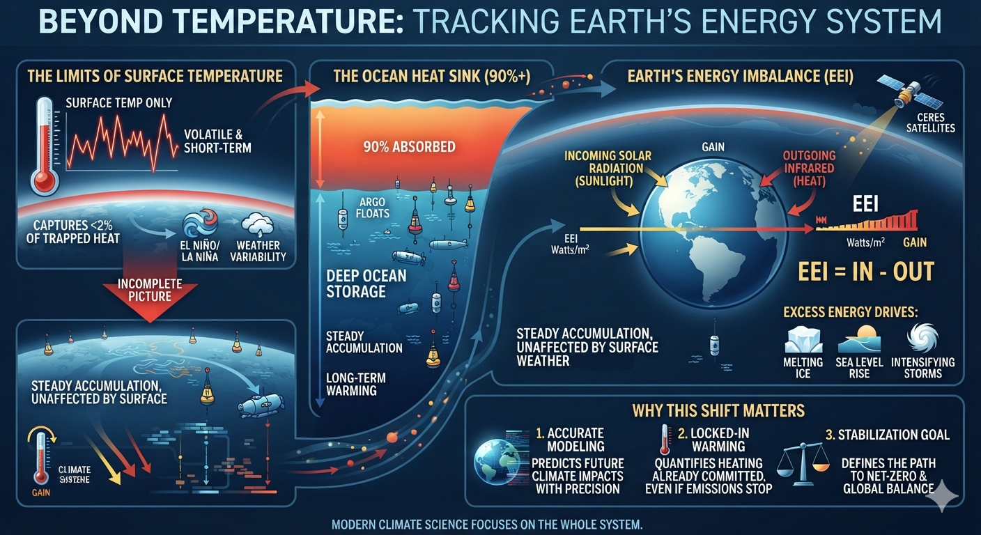
bookmark_borderOzone: The Atmospheric-Ecological Climate Multiplier

Tropospheric Ozone, Carbon-Sink Failure, Wildfire, Lightning, and the Coupled Acceleration of Climate Change

Daniel Brouse¹ and Sidd Mukherjee²

¹Independent Climate Researcher, Economist
²Physicist
Membrane Institute / Philadelphia Spirit Experiment Publishing Company
September 30, 2026

Overview

Ozone represents a rare intersection of climate, ecological, agricultural, and public-health science.

Core Formula

O₃ = Direct Warming + Plant Damage + Carbon-Sink Weakening + Climate Feedback + Atmospheric Coupling

Proposed Central Figure

WARMING

↓

HEAT • DROUGHT • STAGNATION • WILDFIRE • LIGHTNING

↓

OZONE FORMATION

↙         ↘

ATMOSPHERIC    ECOLOGICAL

FORCING      FORCING

↓           ↓

WARMING     VEGETATION DAMAGE

           ↓

       PRODUCTIVITY ↓

           ↓

       CARBON UPTAKE ↓

           ↓

       ATMOSPHERIC CO₂ ↑

           ↓

         WARMING

           ↺

OZONE = ATMOSPHERIC + ECOLOGICAL CLIMATE FORCING

The multiplier is the coupling.


Abstract

Tropospheric ozone (O₃) is commonly treated as an air pollutant and short-lived climate forcer. That description is scientifically correct but incomplete.

Ozone occupies an unusual position within the Earth system because it simultaneously functions as a greenhouse gas, atmospheric oxidant, phytotoxic pollutant, ecosystem stressor, and participant in multiple climate feedbacks. Unlike carbon dioxide, ozone is not primarily emitted directly. It is generated through atmospheric chemistry involving nitrogen oxides (NOₓ), volatile organic compounds (VOCs), carbon monoxide, methane, sunlight, temperature, atmospheric transport, and other chemical processes. Its concentration therefore responds not only to human emissions but also to changing climate conditions.

The central proposition of this paper is the Ozone Feedback Theory:

Tropospheric ozone is an atmospheric and ecological climate-forcing agent that can amplify warming by simultaneously contributing to radiative forcing and weakening biological systems that remove carbon from the atmosphere.

The direct greenhouse effect of ozone is well established. The IPCC Sixth Assessment Report estimates total ozone effective radiative forcing from 1750–2019 at approximately 0.47 W m⁻², with the forcing dominated by tropospheric ozone. This is substantially smaller than the forcing from CO₂, and ozone should not be described as the largest direct greenhouse forcing. Its significance lies elsewhere: ozone couples atmospheric chemistry to vegetation, carbon cycling, hydrology, wildfire, agriculture, human health, and other Earth-system processes.

Recent research strengthens this systems-level interpretation. A 2024 Nature Geoscience study estimated that anthropogenic ozone exposure has reduced tropical-forest net primary productivity and resulted in a loss of approximately 0.29 PgC of annual carbon drawdown since 2000, equivalent to about 17% of the contemporary tropical land carbon sink. A 2024 coupled climate–vegetation–chemistry study found that ozone–vegetation interactions can reduce productivity and stomatal conductance while producing regional warming and drying, particularly in the eastern United States and eastern China. A 2026 Science study found that increasing wildfire emissions reversed previously declining U.S. ozone trends during 2015–2024.

These findings support a broader hypothesis: ozone can function as a climate multiplier because warming can increase conditions favorable to ozone formation while ozone can simultaneously damage vegetation, weaken carbon uptake, increase ecosystem vulnerability, and contribute to further warming.

The resulting system is not a single feedback loop but a network:

Warming → heat/stagnation/fire/lightning → ozone formation → vegetation stress → reduced carbon uptake → atmospheric CO₂ → additional warming

Additional pathways involving methane, wildfire emissions, drought, hydrology, brown carbon, permafrost combustion, and ecosystem decline can couple to this network.

The scientific challenge is therefore not to establish that ozone is “the” dominant cause of climate change. CO₂ remains the dominant long-lived anthropogenic forcing. The challenge is to determine how much ozone-mediated amplification contributes to the observed trajectory of climate change and whether existing Earth-system models adequately represent these coupled biological and atmospheric processes.


1. Introduction

Climate change is often presented as a relatively simple relationship:

Fossil-fuel combustion → CO₂ → warming.

That relationship is fundamental, but it does not describe the complete atmospheric and biological response to combustion.

Combustion simultaneously changes atmospheric concentrations of CO₂, methane, NOₓ, VOCs, carbon monoxide, aerosols, black carbon, and other chemically reactive substances. Some of these compounds directly influence Earth’s energy balance. Others alter atmospheric chemistry. Still others affect the biological systems that regulate carbon, water, and energy exchange between the atmosphere and the land surface.

Tropospheric ozone is unusual because it intersects all three domains.

It is:

  1. a greenhouse gas;
  2. a short-lived climate forcer;
  3. a highly reactive atmospheric oxidant;
  4. a phytotoxic pollutant;
  5. a respiratory pollutant;
  6. a suppressor of plant productivity;
  7. a modifier of stomatal behavior;
  8. a contributor to agricultural losses;
  9. a participant in wildfire-related atmospheric chemistry; and
  10. a potential amplifier of climate feedbacks.

This paper synthesizes the ozone research developed through the Membrane Institute and related work from 2024–2026.

The objective is not simply to repeat the earlier papers. It is to combine them into a single framework and distinguish:

what is established,

what is strongly supported,

what is emerging,

and

what remains a hypothesis requiring further quantitative testing.


2. Ozone Must Be Divided by Altitude

The first distinction is essential.

Stratospheric ozone

Stratospheric ozone forms the protective ozone layer that absorbs biologically damaging ultraviolet radiation.

Tropospheric ozone

Tropospheric ozone occurs in the lower atmosphere, including at ground level.

It is harmful to human health, damages vegetation, participates in photochemical smog, and contributes directly to atmospheric warming.

The two should therefore never be treated as interchangeable.

This paper concerns tropospheric ozone.


3. Ozone Is a Secondary Pollutant and Climate Forcer

Unlike CO₂, ozone is not primarily emitted directly into the atmosphere.

It is produced through chemical reactions involving precursor gases.

A simplified representation is:

NOₓ + VOCs + sunlight + atmospheric chemistry → O₃

Methane and carbon monoxide also participate in the broader chemistry controlling tropospheric ozone.

The actual chemistry is substantially more complicated. Ozone production depends on the chemical regime, precursor concentrations, sunlight, temperature, humidity, atmospheric transport, aerosols, and oxidant chemistry.

This distinction matters because ozone can increase even when direct ozone emissions do not.

A region can therefore experience worsening ozone conditions because of:

  • heat;
  • atmospheric stagnation;
  • wildfire emissions;
  • methane oxidation;
  • transported precursor pollution;
  • changing vegetation emissions;
  • lightning-generated NOₓ;
  • or combinations of these factors.

Ozone is consequently a chemically generated climate pollutant rather than a conventional directly emitted greenhouse gas.


4. The Direct Climate Effect of Ozone

Ozone absorbs outgoing infrared radiation.

It therefore contributes directly to the Earth’s radiative energy imbalance.

The IPCC AR6 assessment estimates the effective radiative forcing associated with total ozone changes between 1750 and 2019 at approximately:

+0.47 W m⁻²

with an assessed range of approximately:

+0.24 to +0.70 W m⁻².

The forcing is dominated by changes in tropospheric ozone.

This establishes an important baseline:

Tropospheric ozone is unquestionably a climate-forcing gas.

The significance of ozone lies in what happens after the molecule interacts with the biosphere.


5. Ozone Is Also a Biological Toxin

Ozone enters plant leaves primarily through stomata. Once inside plant tissues, it participates in oxidative reactions that can damage cellular structures and interfere with photosynthesis.

The consequences include:

  • oxidative stress;
  • cellular damage;
  • reduced photosynthetic efficiency;
  • altered stomatal conductance;
  • reduced carbon assimilation;
  • impaired growth;
  • reduced productivity;
  • increased vulnerability to drought;
  • increased vulnerability to heat;
  • increased susceptibility to pests and disease;
  • and increased mortality under sufficiently severe exposure.

This changes the climate significance of ozone. A conventional greenhouse gas adds radiative forcing.

Ozone can add radiative forcing while simultaneously damaging organisms that remove carbon from the atmosphere.

That dual role is the foundation of the Ozone Feedback Theory.


6. The Carbon-Sink Pathway

The basic biological pathway is:

O₃ ↑

↓

Plant injury

↓

Photosynthesis ↓

↓

Carbon assimilation ↓

↓

Net primary productivity ↓

↓

Carbon sequestration ↓

↓

More atmospheric CO₂

↓

Additional warming

The important distinction here is between gross primary productivity (GPP) and actual net carbon sequestration.

GPP is total photosynthetic carbon fixation. Net ecosystem carbon storage depends on photosynthesis minus plant respiration, decomposition, disturbance, mortality, fire, harvest, and other processes. Consequently, ozone-induced reductions in photosynthesis do not automatically translate one-for-one into atmospheric CO₂ increases. Nevertheless, reducing ecosystem productivity and carbon uptake can weaken an important component of Earth’s natural carbon sink.

This is the pathway that transforms ozone from a short-lived pollutant into a potential participant in long-term climate feedback.


7. The Tropical-Forest Evidence

The strongest recent evidence supporting this part of the theory comes from the 2024 Nature Geoscience study by Cheesman and colleagues. The study combined experimental measurements of ozone sensitivity in tropical tree species with a dynamic global vegetation model. Its central result was that anthropogenic ozone has produced substantial reductions in tropical-forest productivity.

The authors estimated:

  • approximately 5.1% average reduction in tropical-forest NPP under their moderate ozone-sensitivity assumption;
  • losses reaching approximately 10.9% in Asian tropical forests;
  • approximately 0.29 PgC per year of lost carbon drawdown since 2000;
  • approximately 17% of the contemporary tropical annual land carbon sink represented by that lost drawdown.

Anthropogenic ozone is measurably interfering with the productivity of tropical forests and therefore with terrestrial carbon cycling.

This is not merely a theoretical possibility.

It is a modeled estimate grounded in experimentally measured plant sensitivity.


8. Ozone–Vegetation–Climate Coupling

A second major development comes from coupled climate–vegetation–chemistry modeling. Zhou and colleagues (2024) used a climate–vegetation–chemistry model to examine ozone–vegetation interactions.

They found that ozone damage can:

  • reduce GPP;
  • suppress stomatal conductance;
  • reduce transpiration;
  • alter latent heat flux;
  • increase sensible heat;
  • produce warmer and drier conditions in important regions;
  • and alter surface ozone itself.

The study estimated global GPP reduction of approximately:

1.80 ± 0.61 PgC yr⁻¹

or approximately:

4.69 ± 1.56%.

The modeled effects were considerably larger in certain regions.

In the eastern United States, the study estimated:

~20% GPP reduction under high ozone sensitivity

and approximately:

26% reduction in stomatal conductance.

The modeled ozone–vegetation interaction also produced approximately:

+0.33°C surface-air warming in the eastern United States

during the simulated boreal-summer conditions.

Their importance is mechanistic:

Ozone damage to vegetation can alter water and energy exchange in ways that feed back into climate.


9. A Second Ozone Feedback

The coupled model reveals an especially interesting mechanism.

Ozone damages stomatal function.

↓

Stomatal conductance declines.

↓

Transpiration declines.

↓

Latent heat flux declines.

↓

Sensible heat increases.

↓

Surface temperature increases.

The warmer and drier environment can then increase plant stress.

Thus:

Ozone → stomatal suppression → reduced evapotranspiration → warming/drying → additional plant stress

This is not simply a carbon-cycle feedback.

It is a land-surface energy and hydrology feedback.

That distinction is important to the larger Membrane climate framework because it demonstrates how one atmospheric pollutant can simultaneously influence:

carbon + water + energy + atmospheric chemistry.


10. The Ozone Feedback Theory

The central feedback proposed by this research can therefore be written:

Primary ozone feedback

Warming

↓

Heat + stagnation + photochemical activity

↓

Ozone formation ↑

↓

Vegetation injury

↓

Carbon uptake ↓

↓

Atmospheric CO₂ ↑

↓

Warming ↑

↓

Ozone formation ↑

This is a reinforcing feedback. Its strength depends upon:

  • ozone precursor emissions;
  • atmospheric chemistry;
  • temperature;
  • sunlight;
  • moisture;
  • ecosystem sensitivity;
  • vegetation recovery;
  • carbon-cycle dynamics;
  • fire activity;
  • and other feedbacks.

How strongly does ozone-mediated coupling amplify warming under different Earth-system conditions?

That is a measurable scientific question.


11. Wildfire Creates a Major Coupling Pathway

Wildfires connect climate warming to ozone formation. Fire emissions contain:

  • NOₓ;
  • VOCs;
  • carbon monoxide;
  • methane;
  • particulate matter;
  • black carbon;
  • brown carbon;
  • and other reactive compounds.

These emissions can generate ozone both near the fire and far downwind. The 2026 Science study by Deng and colleagues provides particularly important evidence for the United States. Using a 1-km-resolution daily ozone dataset covering 2003–2024, the researchers found that U.S. policy-relevant ozone trends reversed:

2003–2015: −0.65 ppb/year

versus

2015–2024: +0.13 ppb/year.

The authors attributed the reversal primarily to increasing wildfire emissions. They estimated that wildfire emissions offset approximately 3.9 years of progress in ozone mitigation.

This provides an important empirical connection:

Climate-driven wildfire pressure → ozone pollution

rather than merely:

fossil fuel combustion → ozone pollution.


12. The Fire–Ozone–Forest Feedback

Once vegetation is included, the system becomes:

Warming

↓

Drought + heat

↓

Wildfire risk ↑

↓

Fire emissions ↑

↓

Ozone precursors ↑

↓

Ozone ↑

↓

Vegetation damage ↑

↓

Forest resilience ↓

↓

Fire vulnerability ↑

↓

More wildfire

This creates a reinforcing fire–ozone–ecosystem pathway. The ozone component does not operate independently. It becomes coupled to the fire regime.


13. Lightning Adds Another Atmospheric Pathway

Lightning is a major natural source of atmospheric NOₓ. Lightning therefore provides a second potential climate–ozone connection:

Warming

↓

More atmospheric moisture

↓

Stronger convection

↓

More lightning

↓

NOₓ ↑

↓

Ozone production ↑

↓

Additional warming

The relationship is complicated and regionally variable. Lightning also produces hydroxyl radicals (OH), which can accelerate methane oxidation and therefore create a counteracting chemical pathway. Lightning provides an important mechanism through which changing atmospheric dynamics can alter ozone chemistry.

The broader significance is that ozone becomes a coupling molecule connecting atmospheric physics with atmospheric chemistry.


14. Methane Creates a Global Ozone Pathway

Methane represents another important connection. Methane is itself a powerful greenhouse gas. It also participates in atmospheric chemistry that produces tropospheric ozone.

Therefore:

Methane ↑

↓

Ozone production ↑

and

Methane ↑

↓

Direct greenhouse forcing ↑

The interaction does not stop there. Ozone chemistry and hydroxyl-radical chemistry influence methane’s atmospheric lifetime. Thus methane and ozone form part of a coupled atmospheric chemical system.

This means that evaluating a fuel or energy source solely by its CO₂ emissions can omit important atmospheric consequences.


15. Diesel, Natural Gas, and Combustion Pathways

Different combustion systems generate different atmospheric signatures. Diesel combustion tends to generate substantial NOₓ and can therefore contribute strongly to local ozone formation. It can also generate black carbon. Natural gas combustion generally produces less NOₓ than diesel under comparable conditions, but methane leakage and incomplete combustion create another pathway. Methane can persist in the atmosphere long enough to become globally distributed before participating in atmospheric chemistry that contributes to background ozone.

The result is not a simple:

diesel = bad

or

natural gas = good

comparison.

The correct systems analysis is:

Fuel → combustion → CO₂ + NOₓ + VOCs + methane leakage/slip + particles → atmospheric chemistry → ozone + radiative forcing + ecosystem effects

The same principle applies to biofuels.


16. The Biofuel Problem

The term “carbon neutral” can be misleading when applied to combustion-based biofuels without accounting for the complete atmospheric and ecological system. Biogenic carbon may be part of a short carbon cycle, but combustion can still produce:

  • NOₓ;
  • VOCs;
  • carbon monoxide;
  • particulate pollution;
  • ozone precursors;
  • and other climate-forcing compounds.

Land-use change, fertilizer use, transportation, processing, combustion efficiency, and ecosystem impacts also affect the overall balance.

Therefore:

carbon cycling ≠ climate neutrality.

A full assessment must include:

CO₂ + CH₄ + NOₓ + VOCs + ozone + aerosols + land use + ecosystem carbon uptake.

The ozone pathway is one reason a narrow CO₂-only accounting framework can miss important climate effects.


17. Pennsylvania Forests as a Long-Term Observation

The Membrane ozone research began partly from long-term observations of Pennsylvania forests.

The observations reported through this research include:

  • substantial foliage loss;
  • canopy thinning;
  • declining canopy height;
  • premature mortality;
  • and increasing vulnerability to drought, heat, insects, and disease.

Some observations have been described as approximately:

40% multi-year foliage loss

and approximately:

33% reduction in canopy height

in certain monitored old-growth systems since approximately 2003.

Forest ecosystems are exposed simultaneously to:

  • ozone;
  • warming;
  • drought;
  • vapor-pressure deficit;
  • hydrological extremes;
  • insects;
  • pathogens;
  • competition;
  • storms;
  • land-use changes;
  • and other pollutants.

Pennsylvania forest observations provide a long-term case study of compound ecological stress in which ozone is a plausible and independently documented contributor.


18. Ozone and the Amazon

The Amazon illustrates why ozone must be considered within a coupled Earth-system framework.

The Amazon is simultaneously:

  • a major carbon reservoir;
  • a biological carbon sink;
  • a massive source of atmospheric moisture;
  • a regulator of regional rainfall;
  • and a fire-sensitive ecosystem.

Ozone damages vegetation.

↓

Carbon uptake declines.

↓

Vegetation becomes less resilient.

↓

Heat and drought produce greater stress.

↓

Fire vulnerability increases.

↓

Forest loss reduces carbon storage and moisture recycling.

↓

Regional drying can increase.

↓

Further forest stress occurs.

This is the type of coupled system in which ozone can act as one component of a larger tipping cascade.

Ozone can increase the stress load on an ecosystem already exposed to warming, drought, fire, deforestation, and hydrological disruption.

When multiple stressors interact, the combined effect can be nonlinear even if no individual stressor is sufficient to cause collapse.


19. Ozone and the Carbon-Sink Transition

The most consequential possibility raised by this research is not simply that ozone reduces plant productivity.

It is that chronic ecological stress could contribute to the weakening of Earth’s natural carbon sinks.

The general transition is:

Strong carbon sink

↓

Reduced productivity

↓

Reduced resilience

↓

Increased mortality

↓

Fire / decomposition / disturbance

↓

Reduced carbon storage

↓

Carbon neutrality

↓

Potential carbon source

This process is not caused by ozone alone. However, ozone can participate in the early stages by reducing productivity and physiological resilience.

That makes ozone potentially important as a precursor to ecosystem destabilization.


20. The Ozone Multiplier

The combined evidence suggests a useful conceptual distinction. A conventional greenhouse gas primarily changes the energy balance. Ozone does that too. But ozone also changes the biological system that helps regulate atmospheric carbon.

Therefore:

Atmospheric pathway

O₃ → infrared absorption → warming

Biological pathway

O₃ → plant injury → reduced productivity → weaker carbon uptake → more atmospheric CO₂ → warming

Hydrological pathway

O₃ → stomatal suppression → reduced transpiration → altered surface energy/water balance

Wildfire pathway

O₃ → vegetation stress → greater vulnerability → wildfire → ozone precursors → O₃

Methane pathway

CH₄ → ozone chemistry + direct greenhouse forcing

Lightning pathway

Warming → convection/lightning → NOₓ → O₃

Ecosystem pathway

O₃ + heat + drought + pests + disease → declining forest resilience

These pathways can overlap.

That overlap is what makes ozone a climate multiplier.


21. The Expanded Ozone Feedback Network

The entire system can be represented as:

FOSSIL-FUEL / COMBUSTION EMISSIONS

↓

CO₂ + CH₄ + NOₓ + VOCs + CO + PARTICULATES

↓

ATMOSPHERIC CHEMISTRY

Ozone ↑

↓

DIRECT CLIMATE FORCING

Radiative warming

↓

VEGETATION

Photosynthesis ↓

Stomatal conductance ↓

Productivity ↓

Carbon uptake ↓

↓

CARBON CYCLE

Atmospheric CO₂ ↑

↓

CLIMATE

Warming ↑

↓

EXTREME CONDITIONS

Heat + drought + stagnation + fire weather

↓

WILDFIRE

CO₂ + CH₄ + NOₓ + VOCs ↑

↓

Ozone ↑

↓

VEGETATION

Additional stress

↓

ECOSYSTEM RESILIENCE

Decline

↺

This is the central architecture of the Ozone Feedback Theory.


22. Ozone as an Earth-System Coupling Agent

The term climate multiplier is useful because it describes something more specific than simply saying ozone is “important.” Ozone does not need to dominate any individual component of the climate system to have systemic significance. Its importance arises from connectivity.

Ozone connects:

atmospheric chemistry

to

plant physiology

to

carbon cycling

to

hydrology

to

wildfire

to

human health

to

agriculture

to

climate forcing.

This makes ozone a potential Earth-system coupling agent.

That may ultimately be more scientifically useful than ranking ozone against CO₂, methane, or other individual climate agents.


23. The 2026 Copernicus Evidence

The Copernicus Atmosphere Watch 2026 assessment provides a striking contemporary observation.

During the first eight months of 2026, nearly 40% of the global population was exposed to harmful levels of ground-level ozone according to the CAMS analysis. Only approximately 5% of the world’s population experienced ozone conditions classified as “good” in the assessment. Asia experienced the greatest burden, followed by Europe and North America.

The CAMS analysis highlights the interaction of:

  • extreme heat;
  • anthropogenic emissions;
  • wildfire pollution;
  • transboundary atmospheric transport;
  • and ozone chemistry.

CAMS has described this interaction as the “ozone-climate penalty.” This terminology is important because it captures a fundamental asymmetry:

warming can worsen ozone pollution,

while

ozone pollution contributes to warming and ecological damage.

The result is a bidirectional relationship rather than a one-way pollution problem.


24. Transboundary Ozone

Ozone also demonstrates that climate and pollution cannot always be managed within political boundaries. Wildfire smoke and ozone precursors can travel hundreds or thousands of kilometers. A wildfire in Canada can affect air quality in the northeastern United States. Methane emitted in one region can contribute to background ozone formation elsewhere. Industrial emissions can undergo atmospheric chemistry far from their source. The climate system therefore converts local emissions into regional and global consequences.

This is another reason ozone belongs in Earth-system analysis rather than being treated solely as a local air-quality issue.


25. Human Health Is Part of the Same System

The same ozone molecule that damages plant cells can damage human respiratory tissues. Ground-level ozone is associated with:

  • respiratory inflammation;
  • asthma exacerbation;
  • reduced lung function;
  • cardiovascular stress;
  • hospitalization;
  • and premature mortality.

This produces an unusual convergence. The same atmospheric chemistry can simultaneously:

damage forests,

reduce crop productivity,

weaken carbon sinks,

increase human health risks,

and

contribute to warming.

Ozone therefore represents a rare intersection of climate, ecological, agricultural, and public-health science.


26. What the Evidence Establishes

Several components of the ozone framework are already strongly established.

Established

1. Tropospheric ozone is a greenhouse gas.

2. Tropospheric ozone contributes positive radiative forcing.

3. Ozone damages vegetation.

4. Ozone reduces photosynthesis under damaging exposure.

5. Ozone can reduce plant productivity.

6. Ozone affects stomatal conductance and transpiration.

7. Wildfires produce ozone precursors.

8. Wildfire emissions can increase ozone far downwind.

9. Methane chemistry contributes to tropospheric ozone formation.

10. Ozone pollution causes significant human-health impacts.


27. What Is Strongly Supported but Still Quantitatively Uncertain

The evidence now supports a broader and more quantitatively developed picture of ozone as an atmospheric and ecological climate-forcing agent. Multiple studies and modeling frameworks identify measurable pathways through which tropospheric ozone can alter carbon uptake, land-surface energy exchange, wildfire vulnerability, atmospheric chemistry, and ecosystem resilience. The principal remaining uncertainty is not whether these mechanisms exist, but how large their combined effect is across regions, ecosystems, and timescales.

Ozone → Carbon-Sink Weakening

Tropospheric ozone damages photosynthetic tissues, reduces plant productivity, and alters stomatal function. Current estimates indicate that ozone exposure may reduce the global terrestrial carbon sink by approximately 10% to 25% relative to potential capacity, corresponding to roughly 0.4–0.8 PgC per year of carbon that remains in the atmosphere.

Over longer periods, this represents a potentially substantial additional atmospheric CO₂ burden. Some estimates indicate an additional 15–30 ppm of atmospheric CO₂ over a century attributable to ozone-related reductions in terrestrial carbon uptake.

The exact global magnitude remains uncertain because ozone sensitivity varies among species and ecosystems, while carbon-cycle responses also depend on drought, temperature, nutrient availability, mortality, decomposition, fire, and land-use change.

The mechanism itself, however, is increasingly well established:

O₃ exposure → plant injury → photosynthesis/productivity ↓ → carbon uptake ↓ → atmospheric CO₂ ↑


Ozone → Additional Warming

Ozone–vegetation interactions can produce warming through at least two distinct pathways.

The first is the carbon feedback:

O₃ damage → reduced carbon sequestration → additional atmospheric CO₂ → additional greenhouse warming.

Current estimates place the additional global warming associated with this indirect carbon-cycle pathway at approximately 0.05°C to 0.2°C by 2100, depending on assumptions about ozone exposure, vegetation response, and future emissions.

The second is the hydro-climate feedback.

Ozone damages stomatal function and can suppress plant transpiration. Reduced transpiration decreases the transfer of water from vegetation to the atmosphere and reduces evaporative cooling. The resulting redistribution of surface energy can increase sensible heating and alter atmospheric moisture and cloud processes.

In heavily polluted, vegetated regions, modeled ozone–vegetation interactions have produced surface-air-temperature increases of up to approximately 1.5°C under particular conditions.

These regional results should not be interpreted as a global ozone-attributable warming of 1.5°C. They demonstrate that the land-surface response to ozone can be climatically significant where ozone exposure, vegetation, and meteorological conditions interact strongly.


Ozone → Increased Ecosystem Vulnerability

Ozone does not act in isolation.

It interacts with heat, drought, vapor-pressure deficit, pests, disease, and other environmental stresses.

Chronic ozone exposure can damage cellular structures, accelerate foliar senescence, reduce photosynthesis, and impair the ability of plants to regulate water loss.

The result is a reduction in ecosystem resilience.

This creates an important distinction:

Ozone need not directly kill an ecosystem to contribute to ecosystem decline. It can reduce the physiological margin by which an ecosystem withstands other stresses.

This makes ozone particularly important during compound heat-and-drought events.


Ozone ↔ Drought and Vapor-Pressure Deficit

The ozone–drought relationship is not linear.

Under severe soil drought, plants normally close their stomata to conserve water. This can initially reduce ozone uptake and therefore reduce ozone injury.

However, chronic ozone exposure can damage the stomatal apparatus itself.

Under high vapor-pressure deficit (VPD), plants are already under pressure to restrict water loss. Ozone can exacerbate the physiological response, producing larger declines in productivity and vegetation greenness.

The resulting interaction can therefore shift from:

drought → stomatal closure → reduced ozone uptake

toward:

ozone damage → impaired stomatal regulation → greater water stress → additional vegetation damage.

This establishes drought and atmospheric dryness as important modifiers of ozone’s ecological effect.


Ozone → Wildfire Vulnerability

There is not currently a scientifically defensible single percentage describing how much wildfire activity is caused by ozone alone.

Ozone operates as a compounding stressor alongside heat and drought.

Chronic ozone exposure can accelerate foliar senescence, damage vegetation, and increase the availability of dry plant material. When severe ozone exposure coincides with compound heatwave-and-drought conditions, ecosystem vulnerability can increase substantially.

The appropriate formulation is therefore:

Ozone stress + heat + drought → vegetation vulnerability ↑ → available dry fuel ↑ → fire susceptibility ↑

Rather than claiming that ozone directly causes a specific percentage of wildfires, the evidence supports treating ozone as a potential amplifier of fire-season ecosystem stress.


Wildfire → Additional Ozone

The reverse pathway is much more directly measurable.

Wildfires emit large quantities of ozone precursors, including VOCs and NOₓ. When smoke plumes interact with sunlight and urban or industrial emissions, substantial photochemical ozone production can occur.

Observed wildfire smoke events have produced local and regional surface-ozone increases on the order of 20%–30%, with some studies reporting average increases of approximately 21 ppb.

Fire emissions can also make a major contribution to ozone in the remote free troposphere.

The resulting feedback is:

warming/drought → wildfire ↑ → VOCs + NOₓ ↑ → ozone formation ↑ → vegetation stress ↑

The 2026 U.S. evidence provides an important real-world example: increasing wildfire influence was identified as a major factor in reversing previously declining ozone trends.


Climate Change → Lightning NOₓ → Ozone

Lightning is responsible for approximately 10% of the global NOₓ budget, but its atmospheric location makes it particularly important for upper-tropospheric chemistry.

Model projections indicate that lightning-generated NOₓ could increase by approximately 33% under RCP4.5 to 78% under RCP8.5 by 2100.

Projected increases in lightning NOₓ have been associated with additional tropospheric ozone burdens of approximately 29–46 Tg in modeling studies.

This establishes another potential climate–ozone pathway:

warming → stronger convection → lightning ↑ → NOₓ ↑ → ozone ↑

The magnitude of this feedback remains sensitive to the response of convection and lightning to future warming and to the complex chemistry of the upper troposphere.


Ozone ↔ Methane and OH Chemistry

Ozone, hydroxyl radicals (OH), and methane form a tightly coupled atmospheric chemical system.

OH is the dominant atmospheric sink for methane and is responsible for removing the majority of atmospheric CH₄.

Ozone chemistry participates in OH production, meaning that changes in ozone can alter the atmosphere’s oxidative capacity and methane lifetime.

This creates an important chemical trade-off.

Changes in ozone pollution can alter OH availability, while wildfire smoke and other pollutants can suppress OH and temporarily slow methane removal.

Consequently:

O₃ ↔ OH ↔ CH₄

represents another atmospheric pathway through which ozone participates in climate forcing.

The direction and magnitude of the net feedback are chemically complex and cannot be reduced to the simple proposition that more ozone always means faster methane removal.


Ozone → Regional Climate Modification Through Vegetation

Ozone-induced changes in stomatal conductance and transpiration can modify:

  • evapotranspiration;
  • latent heat flux;
  • sensible heat flux;
  • surface temperature;
  • boundary-layer moisture;
  • and potentially cloud formation.

The result is a feedback between atmospheric chemistry and land-surface climate.

This is especially important in heavily vegetated regions where transpiration represents a significant component of the surface energy and water budget.

Thus ozone can affect climate not only by absorbing infrared radiation but also by changing how ecosystems exchange heat and water with the atmosphere.


Ozone → Nonlinear Ecosystem Stress

Evidence increasingly indicates that ozone effects become more consequential when exposure occurs simultaneously with other climate stresses.

The relevant system is therefore not:

O₃ → vegetation damage

but:

O₃ + heat + drought + high VPD + fire + biological stress → ecosystem response

This is particularly important because the response to multiple stresses does not necessarily equal the sum of their individual effects.

Once physiological repair capacity, stomatal regulation, or carbon reserves are exceeded, ecosystem responses can become increasingly nonlinear.


Ozone → Earth-System Model Complexity

Modern Earth-System Models increasingly incorporate coupled atmospheric chemistry, vegetation, and land-surface processes.

Frameworks such as DO3SE attempt to represent ozone damage through accumulated phytotoxic ozone dose and stomatal uptake rather than relying solely on ambient ozone concentration.

This represents an important improvement because plant injury depends on the ozone actually entering plant tissues rather than simply the concentration measured in the surrounding atmosphere.

Nevertheless, substantial uncertainty remains in representing:

  • below-ground carbon cycling;
  • root and mycorrhizal responses;
  • species-specific ozone sensitivity;
  • ecosystem adaptation;
  • compound heat-and-drought stress;
  • vegetation mortality;
  • wildfire interactions;
  • and long-term carbon-cycle feedbacks.

Therefore, the central uncertainty has shifted.

It is no longer simply:

Does ozone affect vegetation?

It is increasingly:

How much does ozone-mediated biological damage alter the trajectory of the coupled climate system?


28. What Remains a Research Hypothesis

The evidence now supports the individual components of the Ozone Feedback Theory sufficiently well that the central research question can be stated more precisely.

The remaining hypothesis is not whether ozone damages vegetation, contributes to radiative forcing, interacts with wildfire, or participates in atmospheric chemistry.

Those mechanisms have substantial observational, experimental, and modeling support.

The unresolved question is whether the combined interaction of these mechanisms produces a quantitatively significant contribution to climate acceleration and ecosystem destabilization at the global scale.

The Ozone Feedback Theory therefore proposes:

Tropospheric ozone can function as a climate multiplier when its direct radiative forcing interacts with carbon-sink weakening, altered land-surface energy and water exchange, wildfire feedbacks, methane chemistry, lightning-generated NOₓ, drought, and ecosystem stress. Under sufficiently strong compound stress, these interactions may become nonlinear and contribute to broader climate-feedback cascades.

The principal research questions are:

1. Carbon-Sink Feedback

How much additional atmospheric CO₂ results from ozone-induced reductions in terrestrial carbon uptake?

Current estimates suggest approximately 0.4–0.8 PgC per year of reduced carbon sequestration, but the global value remains sensitive to ecosystem sensitivity, ozone exposure, and interactions with drought, heat, fire, and nutrient limitation.

2. Global Temperature Feedback

How much additional global warming results from ozone–vegetation interactions?

Existing estimates suggest approximately 0.05°C–0.2°C of additional warming by 2100 through the carbon-cycle pathway, while regional land-surface effects can be substantially larger.

The global aggregate effect requires further constraint.

3. Fire-Feedback Attribution

How much wildfire activity is attributable to ozone-induced vegetation stress?

No single global percentage is currently justified.

The more tractable question is how much ozone contributes to fuel desiccation, foliar senescence, ecosystem vulnerability, and fire susceptibility under compound heat-and-drought conditions.

4. Wildfire-to-Ozone Feedback

How much additional ozone is produced by climate-driven increases in wildfire activity?

This pathway is directly measurable through atmospheric observations and chemical transport models.

The critical question is how this contribution changes as wildfire frequency, intensity, duration, and geographic distribution change under continued warming.

5. Lightning–Ozone Feedback

How important will increasing lightning-generated NOₓ become as anthropogenic surface NOₓ emissions decline?

Projected increases of approximately 33%–78% by 2100, depending on the emissions scenario, suggest that lightning could increasingly offset some surface-emission reductions.

The magnitude of the resulting ozone feedback remains uncertain because it depends on future convective behavior and upper-tropospheric chemistry.

6. Methane–OH–Ozone Coupling

How does changing ozone chemistry alter OH concentrations and methane lifetime under a changing climate?

This question is particularly important because ozone, OH, methane, wildfire smoke, and atmospheric oxidizing capacity are chemically coupled.

The net climate effect cannot be determined from ozone concentration alone.

7. Ozone–Drought–VPD Interaction

At what combinations of ozone exposure, soil moisture, temperature, and VPD does plant stress become strongly nonlinear?

This may prove more informative than defining a universal ozone threshold because plant response depends on both exposure and environmental conditions.

8. Earth-System Model Representation

Do current Earth-System Models adequately represent ozone’s effects on vegetation, carbon cycling, hydrology, and wildfire?

Particular attention should be given to:

  • dynamic stomatal uptake;
  • phytotoxic ozone dose;
  • below-ground carbon processes;
  • species-specific sensitivity;
  • compound heat-and-drought stress;
  • ecosystem mortality;
  • wildfire coupling;
  • and atmospheric chemistry.

9. Nonlinear Exposure Thresholds

At what cumulative ozone doses does plant damage transition from approximately linear physiological stress to nonlinear ecosystem degradation?

Critical ozone-dose thresholds may be more useful than ambient concentration alone because biological damage depends upon uptake, exposure duration, species sensitivity, and environmental conditions.

The frequently observed 40–50 ppb range should therefore be treated as an important exposure regime requiring investigation rather than as a universal tipping-point threshold applicable to every ecosystem.

10. Ecosystem Tipping Cascades

Can chronic ozone stress reduce ecosystem resilience sufficiently to contribute to tipping-point cascades?

The proposed pathway is:

Ozone exposure

↓

Stomatal dysfunction and physiological stress

↓

Reduced productivity and increased water stress

↓

Vegetation mortality / structural degradation

↓

Greater fire vulnerability

↓

Carbon release + ozone-precursor emissions

↓

Additional warming and ozone formation

The critical unresolved question is whether this feedback can become strong enough to shift an ecosystem from a stressed but recoverable state into a persistently degraded state.


The Central Research Problem

The next stage of Ozone Feedback Theory should therefore move beyond asking whether individual ozone mechanisms exist.

The more important question is:

Do the atmospheric, ecological, hydrological, carbon-cycle, wildfire, methane, and lightning pathways combine to produce a measurable nonlinear climate feedback?

If so, the magnitude of that feedback must be quantified.

The research objective is consequently to move from:

Ozone as pollutant

to

Ozone as greenhouse gas

to

Ozone as ecological stressor

to

Ozone as coupled climate feedback

to, ultimately,

Ozone as a potential climate-system multiplier.

The distinction is fundamental.

The existence of the mechanisms is increasingly supported.

Their combined magnitude and potential for nonlinear amplification remain the central research questions.


29. The Central Hypothesis

The research synthesized here leads to the following formal hypothesis:

The Ozone Feedback Hypothesis

Increasing tropospheric ozone contributes to climate-system acceleration through simultaneous direct radiative forcing and indirect ecological forcing, with ozone-induced vegetation stress reducing carbon uptake, altering land-surface energy and water exchange, increasing ecosystem vulnerability, and interacting with wildfire, drought, methane, lightning, and other climate feedbacks. These coupled interactions may amplify climate-system responses beyond the effect of ozone considered as an isolated atmospheric constituent.

The hypothesis predicts that the climate significance of ozone should be evaluated together with interacting Earth-system variables, including:

  • vegetation productivity and mortality;
  • terrestrial carbon uptake and carbon-sink strength;
  • drought and vapor-pressure deficit;
  • wildfire activity and fire emissions;
  • temperature and heat stress;
  • atmospheric stagnation;
  • methane concentration and atmospheric lifetime;
  • hydroxyl-radical (OH) chemistry;
  • lightning and lightning-generated NOx;
  • atmospheric ozone concentration and burden;
  • and ecosystem-level physiological stress.

The hypothesis further predicts that ozone effects may operate through multiple interacting feedback pathways rather than through a single linear mechanism. These include:

ozone → vegetation damage → reduced carbon uptake → increased atmospheric CO₂ → additional warming

ozone + drought/VPD → impaired vegetation function → increased ecosystem vulnerability

heat/drought → wildfire → ozone precursors → increased ozone → additional vegetation stress

warming → increased lightning NOx → increased ozone formation → additional atmospheric and ecological forcing

ozone/OH chemistry ↔ methane lifetime → altered greenhouse forcing

The central research question is therefore not simply whether these individual mechanisms exist. Increasing evidence supports their physical and ecological basis. The more difficult question is how strongly these mechanisms interact, whether their combined effects are quantitatively significant at regional and global scales, and whether nonlinear interactions can produce climate-system acceleration or ecosystem destabilization.

Ozone should therefore not be analyzed as an isolated atmospheric variable. Its climate significance should be evaluated as part of the coupled atmosphere–vegetation–carbon–water–fire–chemistry system.


30. The Membrane Systems Model

The broader Membrane climate framework describes climate change as a nonlinear redistribution of energy through a coupled Earth system. Within that framework, ozone can be treated as an intermediary variable.

A simplified energy–biosphere pathway becomes:

Excess energy

↓

Warming

↓

Atmospheric instability / heat / drought / fire

↓

Ozone formation

↓

Atmospheric radiative forcing

Vegetation damage

↓

Carbon-sink weakening

↓

Additional greenhouse gases

↓

Additional energy retention

↓

Additional warming

The significance is not simply the magnitude of ozone’s direct forcing.

It is the number of feedback pathways that ozone can connect.


31. From Feedback to Domino Effect

A single feedback loop can remain relatively weak. Several coupled feedbacks can produce a different system behavior.

For example:

Ozone

↓

forest stress

↓

wildfire

↓

CO₂ + ozone precursors

↓

warming

↓

drought

↓

additional forest stress

At the same time:

warming

↓

lightning

↓

NOₓ

↓

ozone

And:

warming

↓

permafrost thaw/fire

↓

CO₂ + CH₄

↓

warming

These systems can interact.

That is the Domino Effect:

One feedback changes the conditions controlling another feedback.

Ozone may therefore function as one of the connecting molecules within a broader climate-feedback network.


32. A Climate Hierarchy

The synthesis suggests a useful hierarchy:

Level 1 — Primary forcing

CO₂ and other long-lived greenhouse gases

↓

Level 2 — Secondary atmospheric forcing

Ozone, methane chemistry, aerosols, black carbon and other short-lived climate forcers

↓

Level 3 — Biological feedback

Vegetation productivity and carbon-sink response

↓

Level 4 — Physical feedback

Heat, drought, hydrology, wildfire, ice, permafrost

↓

Level 5 — Coupled feedback

Multiple feedbacks interacting

↓

Level 6 — Potential tipping cascade

One destabilized system increases the probability of destabilizing another

Ozone occupies an unusual position because it participates across several levels.


33. Conclusions

Tropospheric ozone should no longer be considered solely an air-pollution problem.

It is a climate-forcing gas.

It is a biological toxin.

It is an ecosystem stressor.

It is a contributor to agricultural losses.

It is a public-health hazard.

It is produced through atmospheric chemistry involving human emissions and natural processes.

And increasingly, evidence indicates that it participates in coupled climate feedbacks.

The direct greenhouse effect is established.

The vegetation effect is established.

The carbon-cycle connection is increasingly quantified.

The wildfire connection is increasingly observable.

The ozone–vegetation climate interaction is demonstrated in coupled modeling.

The global-scale importance of the problem is illustrated by the 2026 Copernicus assessment showing widespread ozone exposure under conditions of extreme heat and pollution.

The remaining scientific challenge is quantitative:

How much does ozone amplify climate change beyond its direct radiative forcing?

That question cannot be answered by comparing ozone’s radiative forcing with CO₂ alone.

It requires evaluating the entire coupled system.

Ozone → atmosphere

Ozone → vegetation

Ozone → carbon cycle

Ozone → hydrology

Ozone → wildfire

Ozone → methane chemistry

Ozone → lightning/NOₓ chemistry

Ozone → human health

and ultimately:

Ozone → coupled Earth-system feedbacks

The central conclusion of this synthesis is therefore:

Tropospheric ozone is not the largest direct driver of anthropogenic warming. Its importance is that it can simultaneously add warming and weaken the biological systems that remove carbon from the atmosphere.

That combination makes ozone fundamentally different from a conventional greenhouse gas.

It is both:

an atmospheric forcing agent

and

an ecological forcing agent.

When those pathways interact with heat, drought, wildfire, methane, lightning, and declining ecosystem resilience, ozone becomes a plausible climate multiplier and Earth-system coupling agent.


References

Principal External Scientific Sources

Cheesman, A. W., Brown, F., Artaxo, P., et al. (2024). Reduced productivity and carbon drawdown of tropical forests from ground-level ozone exposure. Nature Geoscience, 17, 1003–1007. DOI: 10.1038/s41561-024-01530-1.

Deng, W., Wang, J., Zhou, M., et al. (2026). Fires reverse progress toward ozone air quality standards in the United States. Science, 392, 1088–1092. DOI: 10.1126/science.aed3197.

IPCC. (2021). Climate Change 2021: The Physical Science Basis. Chapter 7: The Earth’s Energy Budget, Climate Feedbacks, and Climate Sensitivity.

Zhou, X., Yue, X., Tian, C., & Lu, X. (2024). Global assessment of climatic responses to ozone–vegetation interactions. Atmospheric Chemistry and Physics, 24, 9923–9937.

Cao, J., Yue, X., & Ma, M. (2024). Simulation of ozone–vegetation coupling and feedback in China using multiple ozone damage schemes. Atmospheric Chemistry and Physics, 24, 3973–3987.

Sitch, S., Cox, P. M., Collins, W. J., & Huntingford, C. (2007). Indirect radiative forcing of climate change through ozone effects on the land-carbon sink. Nature, 448, 791–794.

Lombardozzi, D., Levis, S., Bonan, G., et al. (2015). The influence of chronic ozone exposure on global carbon cycling. Journal of Climate.

Mills, G., et al. (2018). Tropospheric ozone assessment report: Present-day ozone distribution and impacts on vegetation. Elementa: Science of the Anthropocene.

Copernicus / Atmospheric Evidence

Copernicus Atmosphere Monitoring Service. (2026). Atmosphere Watch 2026. Global analysis of atmospheric composition, ozone exposure, extreme heat, wildfire emissions, and transboundary pollution.

Membrane Institute Research

Brouse, D. (2024). The Dangers of Tropospheric Ozone: A Silent Threat to Health and the Environment.

Brouse, D. (2025). The Silent Unraveling of Pennsylvania’s Forests: Ozone Stress, Climate Change, and Resilient Tree Species.

Brouse, D. & Mukherjee, S. (2025). The Domino Collapse of Earth’s Climate Systems: Amazon Rainforest Dieback and the Ozone Feedback Loop.

Brouse, D. & Mukherjee, S. (2025). Runaway Feedbacks and the Collapse of Natural Carbon Sinks: Emerging Evidence From Forests, Permafrost, and Tropospheric Ozone.

Brouse, D. & Mukherjee, S. (2026). Ozone as a Climate Multiplier: Key Coupling Agent in Chemistry–Climate Feedbacks.

Brouse, D. & Mukherjee, S. (2026). The Ozone Climate Feedback: Fossil Fuel Combustion, Methane Emissions, Wildfires, and Ecosystem Degradation as Drivers of Self-Reinforcing Global Warming.

Brouse, D. & Mukherjee, S. (2026). Lightning-Generated Tropospheric Ozone and Earth-System Feedbacks.

Brouse, D. & Mukherjee, S. (2026). Ozone Feedbacks From Carbon Combustion: Tropospheric Ozone, Ecosystem Collapse, and the Failure of Biofuel Narratives.

Brouse, D. & Mukherjee, S. (2026). The Ozone Feedback Theory: Tropospheric Ozone as a Driver of Ecosystem Decline, Carbon Sink Failure, and Climate Acceleration.

Brouse, D. & Mukherjee, S. (2026). Known Ozone: The Climate Change Agent That Damages the Carbon Sink.
Brouse, D. (2026). Introduction to Tropospheric Ozone and Climate Change.

Brouse, D. (2026). Low-Level Ozone: The Invisible Climate Pollutant Threatening Human Health and Accelerating Global Warming.

bookmark_borderHow Is Climate Energy Hitting You? California: Wave to Kelvin

by Daniel Brouse

Chaos Theory Oceanic Teleconnection: Tropical Pacific Energy → U.S. West Coast

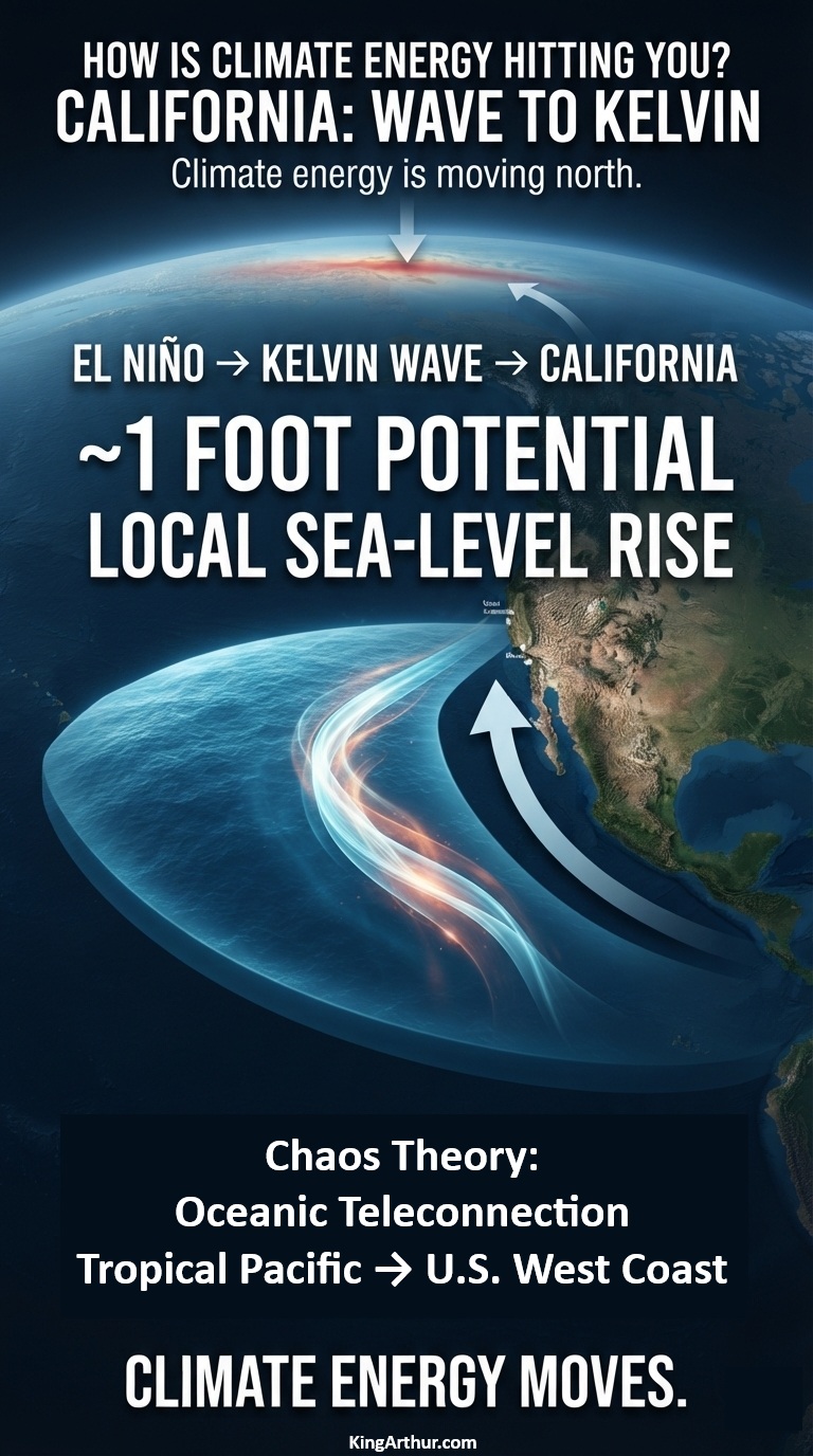
A powerful El Niño is sending a massive pulse of ocean energy north along the Pacific coast—and California could see local sea levels rise by about a foot this fall.

The Weather Channel reports that a coastally trapped Kelvin wave generated by El Niño is moving north toward California and could reach the coast by October 2026, potentially raising local sea levels by about one foot.

That sounds like a giant wave.

It isn’t.

There will be no towering wall of water suddenly approaching the beach.

Instead, scientists are watching a hundreds-of-miles-wide, relatively shallow bulge in the ocean surface—a coastally trapped Kelvin wave carrying energy northward along the Pacific coastline.

And that energy is about to matter.

The Pacific Is Moving Energy North

El Niño changes the normal pattern of tropical Pacific winds.

When the trade winds weaken or reverse, enormous amounts of warm water can accumulate and generate oceanic Kelvin waves. These waves travel eastward across the tropical Pacific. When they reach Central and South America, part of that energy is redirected northward along the coast as a coastally trapped wave.

The result is an extraordinary oceanic connection:

Tropical Pacific → South America → Mexico → California → Pacific Northwest → Alaska

NOAA describes these waves as an important oceanic teleconnection between the tropical Pacific and the U.S. West Coast.

The wave is currently moving north at roughly 6 mph, with the California coastline expected to encounter the advancing disturbance around October.

NOAA: We’ve Already Seen the First Waves

There is an important wrinkle in the story.

NOAA’s September 3, 2026 update says that Kelvin waves generated along the Equator during the spring and summer already reached California in May and June. But NOAA also says those earlier waves are not the main event. According to NOAA Fisheries, their impacts on the West Coast are expected to be minor compared with what may occur during the fall and winter. Scientists are now watching for stronger coastally trapped waves associated with the developing El Niño.

In other words:

California has already received the first pulse.

The larger pulse is coming.

About a Foot of Extra Water

NOAA describes the sea-level effect of these waves as typically being on the order of 15 centimeters—about 6 inches. But that is not necessarily the upper limit of what California can experience during a major El Niño. The Weather Channel’s current reporting puts the potential local sea-level increase from the incoming wave at about one foot.

Why Inches Become Important

A foot of additional coastal water doesn’t have to arrive as a storm surge to cause problems.

It simply makes the starting point higher.

Then add:

  • an exceptionally high tide,
  • large Pacific swells,
  • a coastal storm,
  • low atmospheric pressure,
  • already-rising background sea level,
  • and a coastline that is increasingly exposed to erosion.

The same wave that might have remained below a vulnerable threshold under normal conditions can suddenly push water onto beaches, roads, low-lying neighborhoods and other infrastructure. Higher coastal water also gives incoming waves a higher platform from which to attack beaches, dunes, cliffs and coastal infrastructure.

A Wave You Can’t See Coming

That is what makes the Kelvin wave so interesting. You can’t stand on the beach and see it approaching. It doesn’t have a crest. It doesn’t suddenly break.

The ocean simply becomes higher.

The disturbance can stretch hundreds of miles along the coastline while traveling northward, shifting enormous amounts of ocean water and redistributing energy across the Pacific basin. And because the wave can persist for weeks, its effects can overlap with other coastal hazards. Another wave can even follow behind it.

Climate Energy Doesn’t Stay Put

This is the bigger lesson. Climate energy does not simply accumulate where it first appears.

It moves through the Earth system. A change in tropical Pacific winds generates a Kelvin wave. The wave crosses an ocean. It encounters the Americas. Its energy turns north. The ocean surface rises. Coastal waters warm. Upwelling changes. Storm impacts can become more consequential. And suddenly something that began thousands of miles away in the tropical Pacific is affecting the elevation of the ocean along the California coast.

That’s climate energy hitting you. Not necessarily as hotter air. Not necessarily as a hurricane. Not necessarily as a heat wave. Sometimes it arrives as a foot of extra ocean beneath the next high tide.

Wave to Kelvin

The coming California event is a powerful example of the interconnected nature of the climate system. The first Kelvin waves have already reached California. NOAA says the more significant impacts are expected during fall and winter. The Weather Channel reports that the incoming wave could raise local sea levels by about a foot when it reaches California this fall.

The ocean is carrying energy from the tropics toward the coast.

You won’t see the wave coming.

But you may see what happens when it gets there.

Wave to Kelvin.

bookmark_borderHow Is Climate Energy Hitting You? Hottest Summer Ever: Those Hot Summer Nights

by Daniel Brouse

Simplified Introduction

Tonight’s homework assignment is my favorite: Deep, deep math, statistics, and climate physics.

THE NIGHTTIME HEAT JERK HAS ENTERED A NEW REGIME

The contiguous United States just experienced its hottest meteorological summer on record. But the really interesting signal may be happening after sunset. Summer 2026 averaged 61.71°F for daily minimum temperatures—the warmest summer nighttime average ever recorded.

Nighttime is normally the atmosphere’s recovery period. After sunset, land, pavement, buildings, vegetation, soils, and water can release some of the energy accumulated during the day. But what happens when the recovery period itself starts getting hotter?

That’s where Climate Jerk comes in.

Temperature = the signal.

Warming rate = the first derivative.

Acceleration = the second derivative.

Jerk = the third derivative—the rate at which acceleration changes.

Using a three-period analysis, nighttime-temperature acceleration shifted from approximately −0.4080°F/decade² during the 1990–2010 → 2010–2020 transition to +0.9048°F/decade² during the 2010–2020 → 2020–2026 transition.

That produces an estimated nighttime-temperature jerk of approximately:

+1.14°F/decade³

That does NOT mean temperatures suddenly increased by 1.14°F. It means the behavior of the warming rate changed dramatically. From 2010–2020, the summer nighttime trend was essentially flat. From 2020–2026, it became strongly positive.

The climate system moved from deceleration into substantial acceleration in only six years.

And that matters. The six-year window is especially important because it represents only a fraction of a conventional climate trend period. A change this pronounced over such a short period is precisely why looking exclusively at long-term linear warming can obscure emerging nonlinear behavior. A long-term linear trend tells us where the climate has been going. It may not tell us how rapidly the trajectory is changing right now.

The 2026 nighttime record did not occur in isolation. Much-above-average nighttime minimum temperatures covered most of the contiguous United States, while record nighttime warmth occurred across much of the Southwest.

Meanwhile, the CONUS recorded its hottest meteorological summer ever: 74.4°F, or 3.0°F above the 20th-century average. Think of nighttime heat as thermal memory. A cooler night allows the system to discharge some accumulated energy. A warmer night leaves more energy behind when the next day begins. That can make consecutive hot days increasingly connected rather than independent events.

The most important observation isn’t simply that nights are getting warmer.

It is that the RATE OF CHANGE OF THE RATE OF CHANGE has changed.

And over the last six years, that change has become extreme.

Homework assignment: Do the math.

Then ask yourself what happens when a nonlinear climate system stops merely warming—and starts changing how quickly it warms.


The Nighttime Heat Jerk Is Accelerating

The contiguous United States has just experienced its hottest meteorological summer on record—and one of the most revealing characteristics of the 2026 climate signal is not simply how hot the afternoons became, but how much heat remained after the sun went down.

The National Oceanic and Atmospheric Administration (NOAA) reports that the average temperature across the lower 48 states during June–August 2026 reached 74.4°F, 3.0°F above the 20th-century average. That surpassed the previous summer records set in 1936 and 2021 by 0.4°F.

But averages can conceal the behavior of a nonlinear climate system. To understand what is happening, it is useful to examine nighttime minimum temperatures separately from daytime maximum temperatures.

The Nighttime Heat Factor

Nighttime temperatures are becoming an increasingly important component of the climate system because nighttime is normally a period of thermal recovery. After sunset, the land surface, buildings, pavement, vegetation, soils and water bodies can release some of the energy accumulated during the day.

When nighttime temperatures remain unusually high, that recovery period becomes less effective. The next day begins with a warmer baseline, meaning that the system has less opportunity to dissipate the heat accumulated during the previous day.

A hot afternoon followed by a cool night is therefore one type of heat event. A hot afternoon followed by an unusually warm night, followed by another hot afternoon, is something different: the heat becomes cumulative.

The 2026 summer provides an extraordinary example of this nighttime component of climate energy. The NOAA CONUS June–August minimum-temperature dataset shows a summer average minimum temperature of 61.71°F in 2026, the highest value in the supplied 1895–2026 series.

The Longer-Term Nighttime Signal

The historical data show that nighttime minimum temperatures have not simply risen in a smooth, linear fashion.

For this analysis, the NOAA CONUS June–August minimum-temperature series was divided into three periods: 1990–2010, 2010–2020 and 2020–2026. The purpose is to examine not only temperature change, but the changing rate of temperature change.

The NOAA dataset identifies itself as “Contiguous U.S. June-August Minimum Temperature” and reports the observations in degrees Fahrenheit. The actual summer values show the transition particularly clearly. The 1990 summer Tmin was 59.19°F, while 2010 reached 60.68°F. The 2020 value was 60.64°F, followed by 61.71°F in 2026.

Thus, the nighttime signal did not simply march upward at a constant rate. It slowed during one period and then accelerated sharply during the most recent period.

1990–2010: The Initial Warming Regime

Between 1990 and 2010, the CONUS summer minimum-temperature trend was approximately +0.5774°F per decade.

The actual endpoints were 59.19°F in 1990 and 60.68°F in 2010, while the linear regression across all observations in the interval produces the +0.5774°F/decade trend velocity.

This establishes the first baseline velocity:

V₁ = +0.5774°F/decade

This is warming, but by itself it does not establish acceleration or jerk. It simply tells us how rapidly summer nighttime minimum temperatures were changing during this period.

2010–2020: A Temporary Deceleration

Between 2010 and 2020, the linear trend in CONUS summer Tmin was approximately −0.0345°F per decade. The endpoint values were 60.68°F in 2010 and 60.64°F in 2020.

Thus:

V₂ = −0.0345°F/decade

The 2010–2020 interval represents a slight deceleration—or temporary reversal—in the long-term summer nighttime warming trajectory. That is important because it prevents the analysis from becoming a simple story of uninterrupted acceleration. The climate signal contains variability. A nonlinear system can experience periods of slower change followed by periods of rapid acceleration.

The important question is what happened next.

2020–2026: The Acceleration Returns

The answer is visible in the 2020–2026 data. The 2020 summer minimum temperature was 60.64°F. It then rose to 61.45°F in 2021, 61.21°F in 2022, 60.26°F in 2023, 61.09°F in 2024, 60.87°F in 2025 and 61.71°F in 2026.

The individual years fluctuate, but the linear trend over the seven observations is approximately:

V₃ = +0.6893°F/decade

That is a remarkable reversal from the −0.0345°F/decade trend of 2010–2020.

The 2020–2026 warming velocity is also approximately 19% greater than the +0.5774°F/decade velocity calculated for 1990–2010.

The Nighttime Temperature Jerk

This is where the Climate Jerk framework becomes useful.

A temperature trend describes the first derivative:

V = dT/dt

Acceleration describes the second derivative:

A = d²T/dt²

Jerk describes the third derivative:

J = d³T/dt³

The important question therefore changes from “Are nighttime temperatures getting warmer?” to “Is the rate at which nighttime temperatures are changing itself changing?”

Using the three regression-derived velocities, the transition from 1990–2010 to 2010–2020 produces an acceleration of approximately:

A₁ = −0.4080°F/decade²

The transition from 2010–2020 to 2020–2026 produces:

A₂ = +0.9048°F/decade²

The acceleration therefore changes from negative to strongly positive.

Using the midpoint of each trend interval and calculating the rate of change between those acceleration regimes produces a finite-difference nighttime-temperature jerk of approximately:

J = +1.14°F/decade³

Nighttime Temperature Jerk ≈ +1.14°F/decade³

What the Number Means

The +1.14°F/decade³ value should not be interpreted as though the temperature itself suddenly increased by 1.14°F. It is a third-order rate-of-change measurement.

The first number tells us the temperature is changing. The second tells us whether that temperature change is accelerating or decelerating. The third tells us whether that acceleration is itself changing.

In this analysis, the progression is:

+0.5774°F/decade → −0.0345°F/decade → +0.6893°F/decade

The corresponding acceleration changes from:

−0.4080°F/decade² → +0.9048°F/decade²

That produces:

+1.14°F/decade³ jerk

The significance is therefore not that every year must be warmer than the preceding year. The significance is that the underlying rate of nighttime warming underwent a substantial reversal and acceleration during the 2020–2026 interval. This is consistent with the concept of nonlinear acceleration: the climate system does not have to follow a smooth upward curve for its rate of change to become increasingly consequential.

A Record Summer Nighttime Signal

The 2026 value of 61.71°F is particularly important because it represents the highest June–August CONUS minimum-temperature value in the supplied 1895–2026 dataset. That record arrives after a period in which the nighttime warming velocity had temporarily weakened.

The sequence is therefore more revealing than any single year’s temperature:

1990–2010: +0.5774°F/decade

2010–2020: −0.0345°F/decade

2020–2026: +0.6893°F/decade

The system went from substantial warming, to a period of near-zero change, to substantially faster warming. That is the behavior we are calling nighttime-temperature jerk.

Hot Nights Change the Meaning of a Heatwave

Nighttime temperatures also change the physical meaning of extreme heat. Consider two hypothetical summer days that both reach 100°F. In the first case, the temperature falls to 65°F overnight. In the second, it falls only to 80°F.

The daytime maximum is identical. The thermal burden is not. In the second scenario, the environment begins the next day 15°F warmer. If that pattern persists for several consecutive days, the system has progressively less opportunity to release accumulated heat.

A heatwave should therefore not be viewed solely as a sequence of daytime maximum temperatures. The overnight minimum matters because it determines how much recovery occurs before the next cycle begins. A warming night effectively raises the starting line for the following day.

From Hot Nights to Drought

The nighttime signal is also part of a broader hydroclimatic system involving evaporation, soil moisture and drought. The relentless combination of heat and limited moisture can cause drought to expand rapidly. By September 1, drought conditions covered 59.1% of the contiguous United States.

Heat increases atmospheric demand for moisture. That accelerates evaporation from soils, vegetation, reservoirs and surface water. As soils dry, evaporative cooling can decline, leaving more energy available to heat the land surface.

The feedback becomes:

Heat → evaporation → drying → drought → reduced evaporative cooling → more heat.

The result is not simply a hotter landscape. It is a landscape increasingly vulnerable to additional heat.

The Nighttime Feedback

Nighttime warming adds another component to this process. If the land does not cool sufficiently overnight, the following day begins with elevated thermal energy already present in the system. That can increase heat stress, reduce nighttime recovery and contribute to cumulative thermal loading.

The sequence becomes:

Daytime heat → nighttime heat retention → reduced recovery → warmer starting conditions → greater next-day heat → additional energy accumulation.

This is why nighttime minimum temperatures may be especially useful for detecting changes in the behavior of the climate system. They tell us something about what happens to accumulated energy after the sun disappears.

The Three-Period Signal

The three-period analysis can be summarized numerically:

PeriodSummer Tmin TrendWarming VelocityChange in Velocity
1990–2010+0.5774°F/decade+0.5774°F/decade—
2010–2020−0.0345°F/decade−0.0345°F/decade−0.6119°F/decade
2020–2026+0.6893°F/decade+0.6893°F/decade+0.7238°F/decade

The corresponding accelerations are:

1990–2010 → 2010–2020: −0.4080°F/decade²

2010–2020 → 2020–2026: +0.9048°F/decade²

And the resulting finite-difference jerk is approximately:

+1.14°F/decade³

This is not a claim that the climate system follows a perfect mathematical curve. It is a measurement of how dramatically the estimated nighttime warming rate changed between the three selected periods.

The Night Is Becoming Part of the Heatwave

For generations, the heat of summer was primarily experienced as something that happened during the day. That distinction is becoming increasingly inadequate. The afternoon heat is only one part of the energy balance. The nighttime minimum determines how much of that accumulated energy is released before the next day’s solar heating begins.

When nighttime temperatures remain elevated, the recovery period contracts. When recovery contracts, heat accumulates. When heat accumulates, the next extreme event starts from a higher baseline. And when the rate of nighttime warming itself changes rapidly, the system begins exhibiting the type of nonlinear behavior described by the Climate Jerk hypothesis.

Those Hot Summer Nights

The phrase “hot summer nights” sounds almost harmless.

It isn’t.

A warmer night means less recovery. Less recovery means greater cumulative heat exposure. Greater cumulative heat exposure increases stress on people, ecosystems, water supplies and infrastructure. The 2026 NOAA data provide a particularly striking endpoint to this story: a CONUS June–August minimum-temperature average of 61.71°F, the highest value in the supplied historical series.

More importantly, the trend analysis shows a dramatic change in the rate of nighttime warming. The velocity increased from −0.0345°F/decade during 2010–2020 to +0.6893°F/decade during 2020–2026.

That change corresponds to an estimated acceleration of +0.9048°F/decade² during the most recent transition and an overall finite-difference jerk of approximately +1.14°F/decade³.

So the question is no longer simply:

How hot is it getting?

The more consequential question is:

How quickly is the system changing how quickly it gets hotter?

That is where the jerk matters. Climate energy is not merely raising the temperature. It may be changing the rate at which the temperature changes. And increasingly, the evidence is showing up after the sun goes down.

Conclusion: The Nighttime Heat Jerk Has Entered a New Regime

The most important finding in the nighttime-temperature record is not simply that summer nights are getting warmer. It is that the rate of nighttime warming has changed dramatically during the past six years.

The 2020–2026 interval marks a striking departure from the relatively weak nighttime-temperature change observed during 2010–2020. In the NOAA CONUS June–August Tmin series, the estimated warming velocity shifts from approximately −0.0345°F per decade during 2010–2020 to +0.6893°F per decade during 2020–2026. That is a reversal of direction and an enormous change in the rate of temperature change.

NOAA’s independent 2026 observations reinforce the signal: July’s CONUS average nighttime minimum reached 64.2°F, 3.7°F above the 20th-century average, the warmest monthly average minimum temperature in the record.

This is where the concept of Climate Jerk becomes particularly useful. Temperature is the first-order signal; warming velocity is the first derivative; acceleration is the second derivative; and jerk is the third derivative—the rate at which acceleration changes.

Using the three-period analysis, nighttime-temperature acceleration shifts from approximately −0.4080°F/decade² in the 1990–2010 → 2010–2020 transition to +0.9048°F/decade² in the 2010–2020 → 2020–2026 transition. The resulting finite-difference estimate of nighttime-temperature jerk is approximately +1.14°F/decade³.

The significance of that number is not that temperatures suddenly increased by 1.14°F. They did not. The number describes the changing behavior of the warming rate itself. During 2010–2020, the summer nighttime trend was essentially flat. During 2020–2026, the trend became strongly positive. The system therefore moved from deceleration into substantial acceleration within a remarkably short interval.

The six-year window is especially important because it represents only a fraction of a conventional climate trend period. A change this pronounced over such a short period is precisely why looking exclusively at long-term linear warming can obscure emerging nonlinear behavior. A long-term average can tell us where the climate has been heading; it can be much less informative about how rapidly the trajectory is changing now.

And the 2026 record did not occur in isolation. NOAA reports that much-above-average nighttime minimum temperatures covered most of the contiguous United States during summer 2026, while record nighttime warmth occurred across California, Nevada, Arizona, Utah, New Mexico and Colorado in August. At the same time, the CONUS experienced its hottest meteorological summer on record, with an average temperature of 74.4°F—3.0°F above the 20th-century average.

That combination matters because nighttime heat is effectively a form of thermal memory. A cooler night allows the land and built environment to discharge some accumulated energy. A warmer night leaves more energy in the system when the next day begins. As nighttime temperatures rise, the recovery interval becomes less effective, and consecutive hot days can become increasingly connected rather than functioning as independent events.

The 2020–2026 period therefore represents more than another step upward on a temperature graph. It represents a compression of the nighttime recovery cycle. The climate system is increasingly carrying heat from one day into the next.

That has consequences beyond human discomfort. Persistent nighttime warmth can increase cumulative heat stress, extend cooling demand, reduce ecological recovery and interact with soil-moisture and drought feedbacks. NOAA reported that drought covered 59.1% of the CONUS by September 1, 2026, an increase of more than 10 percentage points from early August.

The broader feedback can be expressed simply:

Heat → evaporation → drying → drought → reduced evaporative cooling → more heat.

Nighttime heat adds another component:

Daytime heat → nighttime heat retention → reduced recovery → higher starting temperature → greater next-day heat → additional heat retention.

This is why the nighttime signal deserves to be treated as an Earth-system variable rather than merely a measure of sleeping comfort.

The evidence does not show a perfectly smooth acceleration. In fact, the 2010–2020 slowdown makes the subsequent acceleration more—not less—interesting. Nonlinear systems do not necessarily accelerate continuously. They can pause, fluctuate, reorganize and then rapidly shift into a new regime. The important observation here is the change in the rate of change.

Over the last six years, that change has become extreme.

The nighttime warming velocity went from approximately −0.0345°F/decade to +0.6893°F/decade. The associated acceleration jumped to approximately +0.9048°F/decade², producing a calculated finite-difference nighttime-temperature jerk of approximately +1.14°F/decade³.

That is the number to watch:

+1.14°F/decade³

It does not mean that every subsequent year will necessarily be warmer than the previous year. It means that, across the selected intervals, the rate at which summer nighttime temperatures are changing has undergone a powerful positive reversal.

And that may be the most important lesson from the hottest summer ever recorded in the contiguous United States.

The climate system is not merely getting hotter.

It is changing how quickly it gets hotter—and increasingly, that change is happening at night.

bookmark_borderHow Is Climate Energy Hitting You? Reno, Nevada

by Daniel Brouse

How Is Climate Energy Hitting You?

Reno, Nevada: Hydroclimatic Whiplash, Flash Droughts, Extreme Winds, and Wildfires

Reno, Nevada, is experiencing some of the most pronounced climate stresses in the American West. Rapid warming is intensifying the region’s existing desert and alpine vulnerabilities, while simultaneously altering snowpack, water supplies, vegetation, wildfire conditions, and extreme precipitation.

For the Reno–Sparks region, the major climate pressures include extreme urban heat, declining Sierra Nevada snowpack, prolonged drought, abrupt swings between wet and dry conditions, extreme winds, flash flooding, and an expanding wildfire season.

These impacts do not occur independently. They interact, creating compound hazards in which one climate extreme can prepare the landscape for another.

Extreme Urban Heat and Season Shifts

Rapid Temperature Increases

Reno has experienced substantial long-term warming, with average temperatures increasing by approximately 7.9°F overall. Average summer temperatures have increased by more than 11°F since 1970, intensifying heat stress across the region.

Urban Heat Island Effect

Rapid population growth has replaced natural landscapes with pavement, buildings, roads, and other heat-absorbing surfaces. The resulting urban heat island effect can substantially increase temperatures within developed areas, placing the greatest burden on residents and communities with fewer resources to adapt.

A Later First Freeze

Reno’s autumn is warming particularly rapidly. The average date of the first winter freeze has shifted later by nearly six weeks, extending the period during which heat-sensitive ecosystems, agriculture, and disease vectors remain active.

Longer Mosquito Seasons

Warmer autumn conditions can delay the seasonal die-off of mosquitoes. In Washoe County, mosquito abundance has increased dramatically, with reports of an eight-fold increase in mosquitoes per trap.

The result is more than a warmer city. The seasonal timing of biological systems is changing.

Snowpack, Water Supply, and Flooding

Diminishing Snowpack

Warming at higher elevations is reducing the amount of winter precipitation stored as snow. Sierra Nevada snowpack has reached exceptionally low levels, at times falling to approximately 48% of the historical median.

Snowpack is not simply frozen precipitation. It is a natural reservoir that stores water through winter and releases it gradually during spring and summer.

Earlier Snowmelt

Warmer winters are shortening the snow season and causing snow to melt earlier. That shifts runoff toward earlier months, leaving less water available during the hot, dry summer period when vegetation, ecosystems, agriculture, and communities need it most.

Lake Tahoe Under Stress

Nearby Lake Tahoe is also responding to a warming climate. Increased thermal stratification can reduce mixing between surface and deeper waters, affecting oxygen distribution, water quality, and ecosystem conditions while creating opportunities for invasive species.

From Drought to Flash Flood

Climate change does not simply mean “more drought.”

A warmer atmosphere can hold more water vapor, increasing the potential for intense precipitation when storms occur. An +11°F increase in temperature equates to an approximate 43% increase in the atmosphere’s maximum capacity to hold moisture. After prolonged dry periods, intense rainfall can produce rapid runoff, flash flooding, erosion, and debris flows across steep mountain terrain.

The same landscape can therefore experience both water scarcity and dangerous excess water—sometimes within a relatively short period.

Wildfires and Public Health

The Invisible Dual Disaster

Reno increasingly faces the convergence of extreme heat and wildfire smoke.

Wildfire smoke can severely degrade outdoor and indoor air quality. During smoke events, poorly sealed buildings and certain cooling systems can allow polluted outdoor air to enter indoor spaces, creating an additional public-health burden precisely when residents are trying to escape the heat.

A Longer Fire-Weather Season

Climate change has contributed to a substantial increase in fire-weather conditions across the region, with estimates of approximately 28 additional fire-weather days annually.

A longer period of hot, dry, windy conditions creates a larger window for vegetation to dry out and fires to spread rapidly.

But temperature alone does not explain the danger.

Water availability, vegetation growth, drought, snowpack, humidity, and wind interact to determine how much fuel is available—and how quickly that fuel can burn.

The Hawk Fire: Hydroclimatic Whiplash in Action

The Hawk Fire, threatening communities northwest of Reno, illustrates how multiple climate and weather processes can converge into a rapidly escalating wildfire emergency.

The fire has expanded dramatically across the Peavine Peak area and threatened residential communities and the University of Nevada, Reno campus. It is occurring amid a broader sequence of major wildfires across northern Nevada.

The immediate fire emergency is being amplified by dry fuels, limited snowpack, extreme fire-weather conditions, and powerful, shifting winds.

This is where the concept of hydroclimatic whiplash becomes important.

Hydroclimatic Whiplash

Hydroclimatic whiplash describes rapid swings between substantially wetter and substantially drier conditions.

The danger is not simply the wet period or the dry period individually.

It is what happens when they occur in succession.

1. Priming the Landscape

An unusually wet period can produce explosive growth of grasses, brush, and other fine fuels.

2. Rapid Dry-Down

If that period is followed by an exceptionally hot and dry summer, the newly produced vegetation can cure rapidly, transforming abundant biomass into highly flammable fuel.

3. Ignition

Once the landscape is sufficiently dry, a single ignition source can rapidly transform a fuel-rich environment into a fast-moving wildfire.

This creates a dangerous sequence:

Wet → Growth → Heat → Drought → Fuel Curing → Ignition → Rapid Fire Spread

The climate hazard is therefore not one isolated extreme. It is the interaction between extremes.

Extreme and Shifting Winds

Wind can turn a dangerous wildfire into an urban emergency.

Powerful red-flag conditions can push flames rapidly across foothills and directly toward residential neighborhoods. At the same time, shifting winds can cause fire behavior to change direction with little warning.

For firefighters, this creates extraordinary tactical difficulties.

Rapidly changing winds can:

  • accelerate fire spread;
  • generate intense fire runs;
  • loft embers ahead of the main fire;
  • ignite new fires across containment lines;
  • block access routes;
  • change evacuation conditions;
  • and place firefighters and equipment in rapidly changing danger zones.

Reports of extreme fire behavior underscore the interaction between wind, dry fuels, topography, and heat.

The result is a wildfire that does not simply spread outward.

It can surge, jump, change direction, and accelerate.

Mitigation and Policy Adaptation

Reno’s climate risks are forcing governments to rethink how cities are designed and how resources are managed.

Heat Mitigation

Nevada’s Assembly Bill 96 establishes requirements for incorporating heat-mitigation strategies into local planning. Measures can include cool roofs, exterior shading, and drought-tolerant landscaping and trees.

These interventions address an important reality: climate adaptation increasingly has to occur at the neighborhood and building scale.

Resource-Demand Feedback

The rapid increase in extreme heat is also increasing pressure on water supplies, electricity demand, energy storage, and grid reliability.

During extreme heat, demand for air conditioning and other cooling systems can rise sharply—at the same time that drought and declining water availability place additional pressure on regional water resources.

This creates a reinforcing feedback:

More heat → More cooling → More electricity demand → Greater grid stress

At the same time:

More development → More water demand → Greater pressure on limited water supplies

These pressures can compound one another. A rapidly growing population and expanding technology sector increase demand for both electricity and water, while extreme heat makes both resources more critical.

Climate adaptation, therefore, cannot be separated from infrastructure planning, resource management, and the capacity of the electric grid and water systems to withstand increasingly extreme conditions.

The Bigger Picture

Reno’s climate challenge is not simply that the city is becoming hotter.

The more important change is that multiple parts of the climate system are beginning to interact in ways that amplify risk.

A warmer atmosphere changes precipitation.

Warmer winters reduce snowpack.

Reduced snowpack changes runoff.

Earlier runoff increases summer dryness.

Summer heat dries vegetation.

Drought converts vegetation into fuel.

Wind accelerates fire.

Wildfire produces smoke.

Smoke threatens public health.

And intense rainfall following dry periods can produce flash floods and debris flows.

This is hydroclimatic whiplash: not merely more extreme weather, but increasingly abrupt transitions between opposing extremes.

For Reno, the question is therefore not simply:

How much warmer will it become?

The more consequential question is:

How will all of these changes interact—and how quickly will they compound one another?

That is how climate energy is hitting Reno.

Hotter. Drier. Windier. More volatile. And increasingly difficult to manage one hazard at a time.

bookmark_borderA Hound’s Nose

Nemo’s Nose Knows

I’ve been thinking about how to describe Nemo’s nose. He’s half Labrador and looks like a golden Lab, but his brain seems to be wired more like a hound.

I’ve had Labs before, and they all loved the water. You couldn’t keep them out of it. Nemo is completely different. He prefers to use the pool as his drinking bowl. He hates getting in the water himself, but he’s an exceptionally astute lifeguard. He keeps a careful eye on everyone, and if your head goes under, he sounds the alarm.

But even more fascinating is his nose. He has the nose—and the sniffing equipment—of a hound. I’ve joked that he can smell through glass.

I’ve been trying to articulate how his senses and brain work. Under normal conditions, I’d say he has average-to-above-average sight, hearing, touch, taste, and smell. But the moment he detects a scent, something changes. His entire mind seems to reorganize around it. Everything else fades into the background, and his nose develops superpowers.

He can seemingly smell something from a mile away. His nostrils twitch toward the wind as his whole muzzle comes alive, his jowls working as though they’re part of some sophisticated sensory apparatus. His head and body don’t move a bit. Completely still. He becomes almost statue-like, as though every muscle is frozen while his nose is doing all the work. He knows exactly where the bunny is, which direction it’s moving, and somehow seems to know where it’s going next.

And then… poof!

In an instant, the stillness explodes. He’s fast as lightning, and suddenly Nemo and the bunny are nothing but a blur.

I imagine his “mind’s eye” as something like scent-a-vision with Dolby Surround Sound—but instead of seeing in colors, he experiences the world in shades and layers of scent.

For Nemo, a scent isn’t just a smell. It’s a picture, a map, a direction, a distance, and a moving story—all unfolding inside his head through his nose.

bookmark_borderThe Good Ancestor and the Climate System: Applying Long-Term Thinking to a Nonlinear Climate Future

by Daniel Brouse

Introduction

Roman Krznaric’s The Good Ancestor: How to Think Long Term in a Short-Term World begins with a deceptively simple question: How can we become good ancestors? His argument is fundamentally about time. Modern societies have become increasingly organized around immediate rewards, quarterly results, election cycles, daily news, and rapidly changing information. The climate system operates on radically different temporal scales. Carbon dioxide released today can influence atmospheric and oceanic processes for decades to centuries, while ice sheets, ocean circulation, ecosystems, and human infrastructure respond through interacting processes that unfold across multiple time horizons.

This temporal mismatch is one of the central problems in understanding climate change.

The climate problem is therefore not merely a problem of atmospheric physics. It is also a problem of human time perception. We make decisions within political, economic, and personal time horizons while the Earth system accumulates energy, reorganizes circulation, alters hydrological patterns, loses ice, and modifies ecological and social conditions over much longer periods.

Krznaric identifies six approaches to long-term thinking: deep-time humility, legacy mindset, intergenerational justice, cathedral thinking, holistic forecasting, and transcendent goal.

Applied to climate science, these six principles provide more than an ethical framework. They provide a conceptual architecture for understanding why conventional climate decision-making repeatedly underestimates systemic risk.

My climate work has focused on a related problem: climate change is not adequately described as a linear increase in average temperature followed by proportionally increasing impacts. The climate system is a coupled, nonlinear system in which accumulated energy can alter the conditions governing subsequent change. Ocean heat, atmospheric moisture, sea-level rise, ice loss, circulation changes, extreme heat, ecological degradation, and socioeconomic disruption interact across different timescales.

The result is a fundamental challenge to short-term thinking.

We are attempting to manage a long-duration, nonlinear Earth-system transition with institutions designed to optimize the present.

Krznaric’s Good Ancestor framework provides a powerful way to confront that contradiction.


1. Deep-Time Humility: Recognizing the Scale of the System

Krznaric’s first principle is deep-time humility: understanding humanity’s extraordinarily small position within the history of Earth and the cosmos. His argument is that recognizing our temporal insignificance can expand rather than diminish our sense of responsibility.

Climate science makes this principle especially important.

Human political systems commonly operate within horizons of months, years, or decades. Climate processes operate simultaneously across days, years, decades, centuries, and longer. An extreme heat event can develop within hours. Ocean heat accumulation occurs over years and decades. Ice-sheet responses can extend over centuries. Carbon-cycle consequences can persist much longer.

These are not competing descriptions of the same phenomenon. They are different temporal layers of one coupled system.

That distinction matters because a climate system can appear relatively stable when observed over one interval while undergoing substantial structural change over another.

A single year’s temperature anomaly tells us something important about the state of the system. But it does not necessarily reveal the direction of the system’s underlying dynamics.

This is why rates of change and changes in rates of change matter.

A climate variable that is increasing linearly presents one kind of risk. A variable whose rate of increase is itself changing presents another. If the acceleration persists, projections based solely on historical averages can systematically underestimate the future trajectory.

The same principle applies to sea-level rise, ocean heat, extreme heat, ice loss, and other indicators. The important question is not simply:

How much has the climate changed?

It is also:

How rapidly is the rate of change itself changing?

This perspective is consistent with the central premise of a nonlinear climate framework: the Earth system must be evaluated not merely by its current state, but by its trajectory, acceleration, feedback structure, and proximity to thresholds.

Deep-time humility therefore changes the unit of analysis.

We stop asking only what climate conditions will look like at the end of the next political cycle and begin asking what trajectory we are establishing for people living decades, centuries, and generations from now.


2. Legacy Mindset: The Climate We Leave Behind

Krznaric’s second principle is the legacy mindset: asking how future generations will remember what we did with the conditions inherited by our generation.

This is particularly powerful when applied to climate change because humanity is not merely experiencing a changing climate.

We are actively determining the initial conditions inherited by future generations.

Every generation receives an Earth system shaped by previous generations and then modifies it before passing it forward.

The critical question becomes:

What climate system are we leaving behind?

That question is larger than carbon emissions alone.

We are leaving future generations altered coastlines, changed hydrological regimes, warmer oceans, different ecosystems, stressed agricultural systems, modified atmospheric circulation, altered wildfire regimes, infrastructure designed for historical climate conditions, and potentially reduced resilience to compound extremes.

The legacy is therefore a system state, not simply an emissions total.

This distinction is important to a nonlinear framework. The consequences of present decisions are not necessarily proportional to the decisions themselves. A system approaching a threshold can respond very differently from one far from a threshold.

The legacy mindset consequently requires us to evaluate not merely the emissions we produce but the conditions under which future generations will have to operate.

That changes the moral question from:

How much climate damage can we tolerate?

to:

What state of the Earth system are we willing to hand to people who had no role in creating it?

That is a substantially different standard.


3. Intergenerational Justice: Future People Are Stakeholders

The third principle, intergenerational justice, asks us to recognize obligations to people who do not yet exist. Krznaric explicitly connects this concept to thinking about the seventh generation and the rights and interests of future people.

Climate change exposes a fundamental weakness in conventional economic and political accounting: the people who receive many of the costs may not be the people making the decisions that generate them.

A decision made today can produce benefits immediately while distributing costs across decades.

That creates a profound temporal asymmetry.

The beneficiaries are present.

The consequences may be inherited.

This becomes even more consequential when nonlinear processes are involved. A generation may consume the benefits of an activity while transferring to future generations a climate system with fewer degrees of freedom and less resilience.

This is the point at which climate science and climate ethics converge.

If the system is approaching thresholds, then delaying action does not simply preserve the same problem for later. It can change the problem itself.

The future may inherit not merely more warming, but a different set of system dynamics.

That distinction is central.

A linear interpretation imagines:

more emissions → proportionally more warming → proportionally more impacts.

A nonlinear systems interpretation recognizes the possibility of:

forcing → warming → feedback amplification → system reorganization → threshold crossing → cascading consequences.

The precise behavior of each component must be established scientifically; not every proposed feedback or tipping interaction is equally certain. But the broader systems principle is robust: interacting components can produce outcomes that are not adequately represented by treating each component independently.

Intergenerational justice therefore demands more than reducing today’s visible damage.

It requires maintaining future adaptive capacity.


4. Cathedral Thinking: Building What We Will Never See Completed

Krznaric’s fourth principle is cathedral thinking: beginning projects whose completion or full benefits extend beyond an individual lifetime. He uses the cathedral as a metaphor for undertaking work whose builders understand that they may never see the finished structure.

This concept fits climate science almost perfectly.

Climate stabilization, ecosystem restoration, adaptation of infrastructure, long-term water management, coastal planning, soil restoration, forest management, energy transformation, and preservation of scientific observations all require decisions whose full consequences extend beyond ordinary political cycles.

But cathedral thinking must go beyond simply building large projects.

It requires building institutional continuity.

A climate strategy designed for four years is not a long-term climate strategy. Neither is one designed around a single election, market cycle, administration, or corporate planning horizon.

The climate system does not reset when political leadership changes.

A genuine cathedral approach would therefore establish institutions capable of maintaining long-term climate observation, infrastructure adaptation, ecosystem protection, scientific research, and risk management regardless of short-term political fluctuations.

This also changes the purpose of climate modeling.

A model should not merely tell us what conditions are likely at a particular future date. It should help identify path dependencies—decisions made today that constrain what future generations can realistically do.

That is especially important when dealing with tipping elements.

If Greenland ice loss, West Antarctic ice instability, permafrost degradation, Amazon ecosystem stress, ocean circulation changes, or other components approach thresholds, the relevant question is not simply whether a particular threshold will be crossed at a particular date.

The more important question is:

Are we constructing conditions that make future reversibility increasingly difficult?

Cathedral thinking therefore demands that we evaluate irreversibility and option value.

A decision that preserves future options has value even if its immediate economic return is difficult to quantify.


5. Holistic Forecasting: From Isolated Variables to a Coupled System

The fifth principle, holistic forecasting, may be the most directly compatible with a nonlinear climate framework.

Krznaric argues that long-term forecasting must consider multiple pathways for civilization rather than rely upon narrow forecasts of a single future.

Climate science requires precisely this kind of thinking.

The Earth system is not a collection of independent variables.

Atmospheric warming influences atmospheric moisture. Increased moisture changes latent heat transport and precipitation dynamics. Ocean warming alters marine heatwaves, circulation, and sea-level contributions. Ice loss modifies albedo and freshwater fluxes. Atmospheric and oceanic circulation redistribute energy. Ecosystem degradation changes carbon storage and surface energy exchange. Extreme events impose stress on infrastructure, agriculture, insurance systems, financial markets, and public health.

These processes can interact.

A useful conceptual chain is therefore not:

CO₂ → temperature → damage.

It is closer to:

forcing → energy accumulation → physical response → feedback → circulation and ecological response → extreme events → infrastructure and economic stress → societal response → additional environmental feedbacks.

This is where the concept of nonlinear acceleration becomes important.

The climate system may exhibit changes in the rate of change because feedbacks alter the system’s effective response over time.

A useful research framework therefore needs to monitor at least four dimensions:

  1. State — where the system is.
  2. Velocity — how rapidly it is changing.
  3. Acceleration — whether that rate is changing.
  4. Coupling — whether independent indicators are becoming dynamically connected.

The fourth dimension is particularly important.

A collection of extreme indicators becomes much more consequential when they cease behaving as isolated anomalies and begin interacting as components of a broader system transition.

This is why the emphasis on persistent nighttime heat, ocean heat accumulation, sea-level acceleration, hydrological disruption, and tipping-system interactions is important.

The question is no longer simply whether one record has been broken.

It is:

Are multiple components of the climate system changing simultaneously in ways that reinforce one another?

That is a holistic forecasting question.


6. Transcendent Goal: From Climate Management to System Preservation

Krznaric’s sixth principle is the transcendent goal—a purpose larger than short-term institutional interests. His formulation points toward the goal of creating conditions in which humanity and the living world can thrive over the long term.

Climate policy frequently becomes trapped in narrower objectives:

  • reducing emissions by a certain percentage;
  • achieving a particular temperature target;
  • meeting a regulatory deadline;
  • protecting a particular industry;
  • minimizing near-term costs.

These objectives are useful, but they can become inadequate when treated as the ultimate goal.

The deeper objective should be preserving a functioning Earth system capable of supporting human civilization and ecological complexity across generations.

That means climate policy should ultimately be judged by resilience rather than by any single metric.

The goal is not merely to minimize today’s inconvenience.

It is to preserve the capacity of future generations to choose their own future.

That is a transcendent objective because it places human civilization within the larger Earth system rather than treating the environment as an externality.


The Six Principles as a Climate Research Architecture

Krznaric’s six principles can therefore be transformed from philosophical concepts into an analytical framework for climate research:

Krznaric principleClimate application
Deep-Time HumilityAnalyze climate trajectories across decades, centuries, and longer system timescales
Legacy MindsetMeasure the Earth-system conditions inherited by future generations
Intergenerational JusticeTreat future adaptive capacity as an ethical and analytical constraint
Cathedral ThinkingDesign climate institutions, infrastructure, and restoration projects beyond political cycles
Holistic ForecastingModel coupled physical, ecological, economic, and social pathways rather than isolated variables
Transcendent GoalPreserve a resilient Earth system and the long-term capacity of civilization to thrive

Together, these principles produce something more powerful than a philosophical appeal to “think long term.”

They provide a temporal systems framework.


From Climate Change to Climate Regime Change

This framework also helps explain why the distinction between climate change and climate regime change matters.

Climate change can be understood as a shift in the statistical characteristics of the climate system.

Climate regime change goes further.

It asks whether the underlying relationships among components of the system are themselves changing.

A regime transition could manifest as persistent changes in extreme heat, nighttime temperatures, precipitation behavior, ocean heat, sea-level rise, circulation patterns, ecological responses, or the frequency and persistence of compound extremes.

The importance of persistent nighttime heat illustrates this distinction.

A daytime temperature record is an extreme event.

Persistent elevation of nighttime temperatures is different because the nighttime period normally provides an opportunity for ecosystems, infrastructure, agriculture, and human bodies to dissipate accumulated heat.

When nighttime cooling is progressively compressed, heat accumulates across successive days.

The system is no longer simply producing isolated extremes.

The baseline itself is moving.

This is precisely where the Good Ancestor framework becomes useful.

A short-term observer asks:

Was today unusually hot?

A long-term systems observer asks:

Has the system entered a state in which unusually hot conditions are becoming persistent, self-reinforcing, and structurally normal?

Those are fundamentally different questions.


The Climate Problem as a Failure of Temporal Governance

Krznaric describes modern society as being dominated by what he calls the “tyranny of the now”: the tendency to privilege immediate concerns over long-term consequences.

Climate change exposes this problem with unusual clarity.

Political systems are optimized around elections.

Businesses are often optimized around quarterly or annual performance.

Financial systems discount future returns.

News systems reward immediacy.

Social media rewards attention measured in seconds.

The climate system does not operate according to any of these clocks.

This produces a structural mismatch:

Human institutions optimize for the present while the Earth system integrates the past and determines the future.

That mismatch is one reason climate risks can repeatedly be underestimated.

A society may respond to an extreme event after it occurs while failing to recognize that the event is part of a changing distribution.

It may repair infrastructure to the historical climate standard even while the climate distribution is shifting.

It may calculate the immediate cost of mitigation while ignoring the potentially much larger cost of reduced future resilience.

And it may treat each extreme as an independent disaster rather than examining whether multiple extremes are manifestations of a common systemic transition.

Good Ancestor thinking challenges this institutional short-termism directly.


Toward a Good Ancestor Climate Index

The philosophical framework suggests a possible extension of climate-risk measurement.

Instead of evaluating climate policy solely through emissions, temperature, or economic cost, a Good Ancestor Climate framework could ask whether present decisions increase or decrease the resilience inherited by future generations.

Such an assessment could consider:

Physical trajectory:
Are major climate indicators accelerating, stabilizing, or decelerating?

Feedback exposure:
Are positive feedbacks becoming stronger or more interconnected?

Threshold proximity:
Are critical Earth-system components moving toward states where reversibility becomes increasingly difficult?

Persistence:
Are extreme conditions becoming more persistent rather than merely more intense?

System coupling:
Are climate, ecological, infrastructure, economic, and social stresses becoming increasingly interconnected?

Adaptive capacity:
Are we expanding or consuming the ability of future generations to respond?

Intergenerational burden:
Are present benefits being purchased by transferring disproportionate costs into the future?

This would shift climate assessment from a narrow accounting of emissions toward a broader accounting of system inheritance.

The central metric becomes:

What are we leaving behind?


The Good Ancestor Test

Krznaric’s philosophy ultimately suggests a remarkably simple test for climate decisions.

Before making a decision, ask:

Would the people living with its consequences a century from now regard us as responsible ancestors?

That question can be applied to virtually every major climate decision.

Would future generations regard us as good ancestors if we knew that climate indicators were accelerating and chose to treat them as static?

Would they regard us as good ancestors if we knew that physical systems were becoming increasingly coupled but continued to govern them separately?

Would they regard us as good ancestors if we optimized infrastructure for a climate that no longer exists?

Would they regard us as good ancestors if we transferred enormous adaptation costs to people who had no voice in the decisions that created them?

And perhaps most importantly:

Would they regard us as good ancestors if we possessed evidence of an approaching systemic transition but refused to think beyond the next election, fiscal year, or news cycle?

These questions transform climate change from an abstract environmental problem into a question of historical responsibility.


Conclusion

Roman Krznaric’s The Good Ancestor provides an ethical and philosophical framework for confronting one of the greatest weaknesses in modern climate governance: our inability to think on the same temporal scale as the system we are changing.

His six principles—deep-time humility, legacy mindset, intergenerational justice, cathedral thinking, holistic forecasting, and transcendent goal—can be mapped directly onto the requirements of nonlinear climate analysis.

Deep-time humility expands the temporal horizon.

Legacy mindset forces us to consider the Earth system we leave behind.

Intergenerational justice recognizes future people as legitimate stakeholders.

Cathedral thinking requires projects and institutions that outlast their creators.

Holistic forecasting demands that climate risks be evaluated as coupled systems rather than isolated variables.

And the transcendent goal establishes a purpose larger than immediate economic or political interests: maintaining a resilient Earth system capable of sustaining future generations.

This perspective reinforces a central proposition of nonlinear climate research:

The most important climate signal may not be the magnitude of change at a particular moment, but the changing dynamics of the system itself.

If rates of change increase, if feedbacks strengthen, if extremes become persistent, if previously separate components become coupled, and if thresholds become increasingly consequential, then the climate problem is no longer adequately described as a gradual environmental trend.

It becomes a system transition.

And once the problem is understood as a system transition, the moral question becomes unavoidable.

We are not merely deciding what kind of climate we will experience.

We are deciding what kind of Earth system we will hand to those who come after us.

That is the essence of the Good Ancestor principle.

The test of our generation will not ultimately be whether we correctly predicted every detail of the future.

It will be whether, having recognized the direction and dynamics of the system, we acted as though future generations mattered.

In that sense, becoming a good ancestor is not an exercise in nostalgia or moral sentiment.

It is a demand for better temporal mathematics, better systems thinking, better governance, and better stewardship.

The future is not simply something that happens to us.

We are its ancestors already.

bookmark_borderExtreme Energy Event: Violent Rain

“Climate change is increasing the amount of energy violent rain events contain, amplifying how much damage they can inflict.”

The physics of wind and rain are important to understand: their destructive force increases nonlinearly with velocity and is further amplified by density and mass. Even relatively small increases in wind speed or rainfall intensity can produce disproportionately larger impacts and damage.

This principle applies to all extreme energy events. At its core, climate change is an energy imbalance. As excess heat accumulates within the Earth system, more energy becomes available to drive storms, floods, droughts, heatwaves, and wildfires. As the energy intensifies, so do its manifestations.

bookmark_borderBeyond Temperature: How Climate Science Shifted from Measuring Warming to Tracking Earth’s Energy System

Introduction

2023 was a record year for global average surface temperature according to the major observational datasets. However, climate science moved beyond focusing primarily on annual temperature records years ago because, by itself, average surface temperature provides only a limited view of the state of the climate system.

Temperature is an important indicator, but it is only one expression of energy. A changing climate is fundamentally an energy problem: how much energy is entering the Earth system, how much is leaving, and how that excess energy is redistributed among the atmosphere, oceans, cryosphere, and biosphere.

By 2023, climate analysis had increasingly shifted toward tracking total energy accumulation (measured in joules) and understanding how that energy moves through the Earth system. As the climate becomes more nonlinear, individual indicators become less informative when viewed in isolation because many components of the system are beginning to exhibit accelerating and threshold-driven behavior.

Global Warming Is Only the Beginning

The phrase “global warming” is often misunderstood. While it accurately describes rising average surface temperatures, it can understate the broader transformation occurring within the climate system.

The central issue is not simply that the planet is warmer. The issue is that greenhouse gases have created a persistent energy imbalance, causing the Earth system to accumulate and redistribute additional thermal energy.

Global warming is the beginning of climate change—not its endpoint.

Once excess heat is trapped by greenhouse gases, it does not remain as a simple increase in temperature. That energy is transformed into multiple forms throughout the Earth system:

  • Kinetic energy — contributing to stronger winds, changing atmospheric circulation, and more energetic storm systems.
  • Gravitational potential energy — increasing atmospheric instability, vertical convection, and the potential for heavier precipitation events.
  • Latent heat — providing additional energy for hurricanes, atmospheric rivers, and extreme rainfall.
  • Radiant energy — increasing infrared energy retention and amplifying greenhouse feedbacks.
  • Chemical energy — influencing wildfire combustion, carbon cycling, and ecosystem feedbacks.
  • Electrical energy — contributing to increased lightning activity within more energetic convective systems.
  • Mechanical work — accelerating coastal erosion, glacier movement, ocean mixing, and other physical processes.

More than 90% of the excess heat trapped by greenhouse gases is absorbed by the oceans. This stored energy creates long-term consequences because the oceans have enormous thermal inertia. Even if atmospheric emissions decline, previously accumulated heat continues to influence climate behavior.

The Limits of Temperature Alone

Climate modeling is not focused primarily on average surface temperature. Surface temperature is one indicator, but it represents only a small part of the broader Earth system.

The significance of 2023–2024 was not simply that temperature records were broken. It was that multiple climate indicators showed simultaneous changes across the system.

The El Niño–Southern Oscillation (ENSO) cycle is an important example. During El Niño events, the ocean can release large amounts of stored heat into the atmosphere, temporarily amplifying surface temperatures. But the larger scientific question is how that additional energy interacts with other components of the climate system.

This period represented an important shift in climate analysis: moving beyond studying direct human emissions alone and toward understanding the combined influence of human forcing and coupled Earth-system feedbacks.

The focus expanded from:

“How much carbon dioxide are humans adding?”

to:

“How does the Earth system respond once that additional energy begins interacting with interconnected feedback mechanisms?”

From Climate Change to Climate Acceleration

One of the clearest examples of coupled feedbacks emerged during the Canadian wildfires. These events demonstrated the interaction between wildfire emissions, carbon release, vegetation loss, and changes in surface albedo.

When forests burn, they release stored carbon while also reducing the ability of ecosystems to absorb future carbon. Darkened landscapes can absorb more solar energy, creating additional warming effects. These processes interact rather than operate independently.

The result is a climate system where impacts can become increasingly visible at local and regional scales—effectively becoming observable “out your window.”

This does not mean that every individual weather event is caused by climate change alone. Rather, it reflects a growing understanding that a warmer, more energetic climate changes the background conditions in which extreme events develop.

Crossing Thresholds in a Nonlinear System

By 2025, global temperatures exceeded the long-recognized 1.5°C threshold. To a casual observer, a 1.5°C increase may appear small. In a nonlinear system, however, small changes in average conditions can produce much larger changes in physical processes.

Additional warming alters:

  • temperature gradients,
  • pressure differences,
  • atmospheric moisture capacity,
  • ocean circulation,
  • convection patterns,
  • and energy transfer throughout the climate system.

The result is not simply more “warm weather.” It is a more energetic system capable of producing increasingly extreme energy events.

Extreme storms, atmospheric rivers, marine heatwaves, wildfire outbreaks, and precipitation extremes are not merely isolated weather anomalies. They are manifestations of energy moving through an increasingly altered Earth system.

Understanding Climate Change in Terms of Energy

The future of climate science requires looking beyond a single number on a thermometer.

Temperature tells us what the system is expressing.

Energy tells us what is driving the system.

To understand climate change, we must think not only in degrees Celsius, but in joules—and in how those joules move through an interconnected planetary system.

The central question is no longer simply:

“How much has the planet warmed?”

The deeper question is:

“Where is the energy going, how is it being transformed, and what feedbacks are being activated as the Earth system responds?”

bookmark_borderNo Sudden Extinction Jump: But a Strongly Constrained High-End Warming Envelope

by Daniel Brouse and Sidd Mukherjee

Climate Change Scenarios 101

Q: Is climate change extreme and alarming?
A: Yes.


Q: Is a single abrupt climate shift likely to trigger immediate human extinction or a sudden global “die-off”?
A: No. But the system behavior is still highly nonlinear and increasingly constrained by physical limits.

1) Near-term physical upper bound (~9°C warming range)

A useful way to frame the system is that there is an effective upper envelope on near-term warming over the next century or two, shaped by:

  • Radiative forcing saturation limits (logarithmic response of CO₂ forcing)
  • Ocean heat uptake capacity and thermal inertia (the oceans absorb >90% of excess heat, slowing atmospheric response)
  • Atmospheric physics constraints (energy balance limits on how fast surface temperature can diverge globally)
  • Feedback activation timing (many carbon-cycle and albedo feedbacks unfold over decades to centuries, not instantaneously)

Taken together, these factors produce a practical near-term upper bound on the order of ~9°C warming over the next century or two, assuming extreme but physically plausible feedback participation and sustained forcing.

This does not mean certainty—it defines a physical envelope, not a prediction.

Within that envelope, plausible scenario ranges remain:

  • Linear or weak-feedback estimates: ~3–5°C
  • Strong-feedback scenarios: ~6–9°C (upper-range outcomes under sustained positive feedback participation)
  • Long-horizon Earth system outcomes (>2+ centuries): >10°C is possible in some “Hothouse Earth” style frameworks, but not as a rapid near-term transition

With current trajectories and acceleration-based interpretations of forcing growth, the highest probability cluster remains roughly ~4–7°C this century, with uncertainty widening rapidly beyond that.


2) Tipping points: real, but not instantaneous synchronized collapse

We are already observing multiple systems approaching critical thresholds:

  • Amazon rainforest resilience stress
  • Arctic amplification and permafrost carbon vulnerability
  • Greenland and West Antarctic ice sheet destabilization signals
  • Ocean circulation weakening risk

These are best understood not as a single chain reaction, but as a network of interacting nonlinear systems.

Yes—cascading interactions are possible, and some feedbacks can reinforce others. However:

  • They do not occur on a synchronized timetable
  • They unfold over decades to centuries
  • They vary significantly in response time and sensitivity

So rather than a single abrupt planetary “flip,” the more physically consistent picture is:

A multi-century cascade of destabilizing subsystems, with overlapping thresholds rather than a single global singularity event.


Conclusion

Climate change is already extreme and accelerating in impact, and the system is increasingly nonlinear.

But the key distinction is this:

  • Not a sudden global extinction jump
  • Not a single-step runaway to infinity
  • But a bounded physical system (~few °C to upper ~9°C near-term envelope)
  • with compounding, cascading risks distributed across time

The danger is not one abrupt cliff—but a widening band of increasingly unstable trajectories within a physically constrained but still highly disruptive climate system.

Bottom line: We cannot control the laws of physics, but we can control the amount of heat-trapping gases we add to the atmosphere. The most effective action is to phase out fossil fuel combustion as quickly as possible.


What Is Collapse?

Let’s lower the bar then to civilization collapse and define the term. Not talking about timeframes, could you explain what that term means to you? What are some of the things that would happen? How could we recognize the start? What things would fail?

Good question. To me, civilization collapse does not mean humanity suddenly disappears. It means that the interconnected systems that support modern civilization can no longer function reliably over large regions.

Some indicators would include:

  • Chronic food insecurity as repeated crop failures and water shortages overwhelm agricultural adaptation.
  • Persistent disruptions to energy, transportation, and global supply chains.
  • Insurance and financial markets retreating from high-risk regions because losses become unmanageable.
  • Large-scale migration driven by heat, drought, flooding, sea-level rise, and ecosystem decline.
  • Governments increasingly shifting resources from development to emergency response and disaster recovery.
  • Public health systems struggling with heat illness, infectious diseases, poor air quality, and malnutrition.
  • Escalating conflicts over food, water, land, and migration.

I don’t think collapse begins with a single dramatic event. It starts when extreme events become so frequent that societies spend more time recovering than adapting. The warning sign is when critical systems lose resilience and repeated shocks outpace our ability to rebuild.

Some of those early indicators are already observable today. The question isn’t whether civilization stops overnight, but whether enough interconnected systems begin failing simultaneously that they reinforce one another. That’s why many researchers focus on cascading risks and coupled feedbacks rather than isolated events.

When Is Collapse?

There isn’t a universally accepted temperature threshold at which civilization “collapses.” Civilization is an emergent property of interconnected human and natural systems, not a single physical variable.

My argument isn’t based on a hard cutoff like “X°C = collapse.” It’s based on the increasing probability of systemic failure as multiple risks become coupled. Climate science provides the physical forcing, while ecology, economics, engineering, public health, and history help us understand how societies respond to repeated, compounding shocks.

That’s why we use a probabilistic, ensemble-based approach rather than deterministic predictions. We aren’t claiming to know the exact year or exact temperature at which civilization fails. We’re evaluating the likelihood that interacting stresses—food and water insecurity, ecosystem degradation, infrastructure failures, migration, financial instability, conflict, and public health crises—begin reinforcing one another faster than societies can adapt.

History shows that civilizations rarely collapse for a single reason. They typically experience multiple interacting pressures that erode resilience over time. Our work extends that systems perspective to a globalized civilization operating within a rapidly changing climate.

In fact, I would argue that we’re already seeing early signs of self-reinforcing societal feedbacks at approximately 1.5°C of warming. Rising disaster costs strain insurance markets, infrastructure, and government budgets. Food and water insecurity contribute to migration and political instability. Repeated extreme events reduce resilience, making recovery from the next disaster more difficult. These interacting pressures don’t constitute “collapse” by themselves, but they are consistent with the early stages of a cascading systemic process.

We also know that the climate system has substantial thermal inertia. The heat already stored in the oceans will continue influencing the climate for decades, even as emissions are reduced. That means many climate impacts will continue to intensify before stabilizing, extending both the duration of environmental stress and the societal challenges associated with adaptation.

So I would frame it less as “civilization collapses at 4°C or 6°C” and more as “the probability of cascading, systemic disruption increases as nonlinear climate and societal feedbacks intensify.” The exact threshold isn’t the point; the trajectory and the growing interconnectedness of the risks are.

Ecofascism

I think we’re already seeing early-stage societal feedbacks emerge. I’m not saying civilization has “collapsed,” but that some of the reinforcing dynamics associated with systemic decline are becoming visible. Financial stress from repeated disasters, insurance retreat, food and water insecurity, migration, political polarization, and declining institutional resilience don’t occur in isolation—they increasingly interact and amplify one another.

One example that concerns me is the emergence of ecofascist narratives. Ecofascism reframes environmental crisis through an authoritarian lens, portraying environmental degradation as justification for exclusion, coercion, or the suffering of groups considered expendable. Rather than focusing on reducing emissions and building resilience, it redirects the conversation toward hierarchy and scapegoating.

Whether we ultimately call this the beginning of “collapse” is partly a matter of definition. What matters to me is recognizing that climate, ecological, economic, and social systems are increasingly coupled. As those feedbacks strengthen, the probability of cascading disruptions rises, even though the exact trajectory remains uncertain.

Ecofascism and Denialism 101


* Our conclusions are based on decades of research and the development of a probabilistic, ensemble-based climate model that incorporates complex socioeconomic and ecological feedbacks within a dynamic, nonlinear Earth system. Rather than assuming simple linear warming, the model examines how interacting feedbacks can accelerate change and produce a range of plausible futures.

We examine how human activities—deforestation, fossil fuel combustion, industrial agriculture, land-use change, and resource consumption—interact with Earth system processes such as carbon cycling, thermal energy redistribution, the hydrological cycle, biodiversity loss, and disease ecology. These interactions do not behave as simple cause-and-effect relationships. They create interconnected, self-reinforcing feedback loops that can produce abrupt, system-wide changes as thresholds are crossed.

Our current assessment is that the climate system is entering a phase where compound, cascading disruptions become increasingly likely, with climate, ecological, economic, and societal stresses reinforcing one another. We also continually compare our work with observations and the research of other scientists, including James Hansen, whose recent analyses likewise point to a faster pace of warming than many earlier projections.


Note From the Author

It’s an interesting balance in social media land. On one side are the denialists; on the other, the doomers. Ironically, the doomers can end up reinforcing the denialists—if extinction is framed as inevitable, then “what difference does it make?” becomes a permission structure to disengage or even to “party like there’s no tomorrow.”

In that sense, both extremes often stop short of engaging with the underlying physics, atmospheric chemistry, economics, and nonlinear feedback dynamics. Each becomes entrenched in its own ideological loop, which then reinforces itself.

The key point is straightforward: we cannot change the laws of physics, but we can control how much heat-trapping gas we add to the atmosphere. The most effective lever we have is to phase out fossil fuel combustion as rapidly as possible.

bookmark_borderClimate Change and Flood Insurance

In the 1990s, what was considered a 500-year flood was expected to occur, on average, once every five centuries. By the early 2000s, many of those same events were being reclassified as 100-year floods. By the 2020s, they increasingly resembled 10-year floods. Today, in some regions, comparable flood events are occurring every few years.

The flood itself did not change.

What changed was the climate system.

The Big Picture

Short-term stream gauge records can be heavily skewed by sampling variability, and it is absolutely true that local flood “return period” estimates can change significantly as more data are collected. That is basic hydrology.

But that is not the same as what is happening in the climate system.

We are not dealing with a single river gauge with a short record. We are dealing with thousands of independent observational datasets across independent physical domains—temperature, ocean heat content, atmospheric moisture, cryosphere mass balance, sea level rise, and precipitation extremes—all showing consistent directional change.

That is exactly why climate attribution studies and statistical detection work have been able to identify signals with high confidence across multiple decades and datasets.

On the policy side, agencies such as FEMA and others involved in risk modeling (including mortgage and insurance regulators) have updated flood maps, pricing assumptions, and risk frameworks over time. But that reflects evolving hazard conditions and improved modeling—not a refutation of climate-driven trends.

So the key distinction is this:

  • A local statistical revision in a limited dataset
  • Climate science is based on global, physically consistent, multi-variable observational convergence

They are not equivalent statistical problems.

Flood Insurance Policy

In the early 2000s, I met with representatives from FEMA and Fannie Mae. I went into that meeting assuming there was relatively little institutional movement toward aggressive long-term risk mitigation or structural adaptation.

I was pleasantly surprised.

At that time, FEMA had already begun shifting toward a more proactive risk-management framework, including elements of what is now often described as managed retreat in high-risk areas. There was a clear recognition that some locations face recurring or escalating flood exposure, and that long-term resilience cannot rely solely on repeated reconstruction in place.

A significant part of their effort was also focused on education—helping homeowners, lenders, and local governments understand how the U.S. flood insurance system actually works, including its limitations. Many people are still unaware that standard coverage is constrained by caps, exclusions, and policy limits that may not fully reflect total rebuilding costs, especially over the lifetime of a property.

The broader goal, as it was explained to me, was not just insurance pricing, but reducing systemic exposure over time through a combination of improved mapping, risk communication, and gradual migration away from the highest-risk zones where feasible.