bookmark_borderThe Nonlinear Acceleration of Climate Change: Feedback Coupling, Tipping-Point Cascades, and the Emerging Climate-Economic Singularity

An Integrated Earth-System and Economic Risk Framework

By Daniel Brouse¹ and Sidd Mukherjee²
November 14, 2026

¹ Independent Climate Researcher and Economist, Membrane Institute, USA
² Independent Physicist, Membrane Institute, USA


Abstract

Climate change is transitioning beyond a predominantly emissions-driven process into an increasingly interconnected Earth-system disturbance characterized by nonlinear acceleration, reinforcing feedbacks, interacting tipping points, and cascading consequences. The implications extend beyond environmental change into the economic, financial, ecological, and institutional systems upon which civilization depends.

This paper integrates the collaborative research of Daniel Brouse and Sidd Mukherjee, building upon their Nonlinear Acceleration Hypothesis, developed in the late 1990s, and subsequent investigations into climate feedback coupling, third-derivative behavior, tipping-point networks, and climate-economic instability.

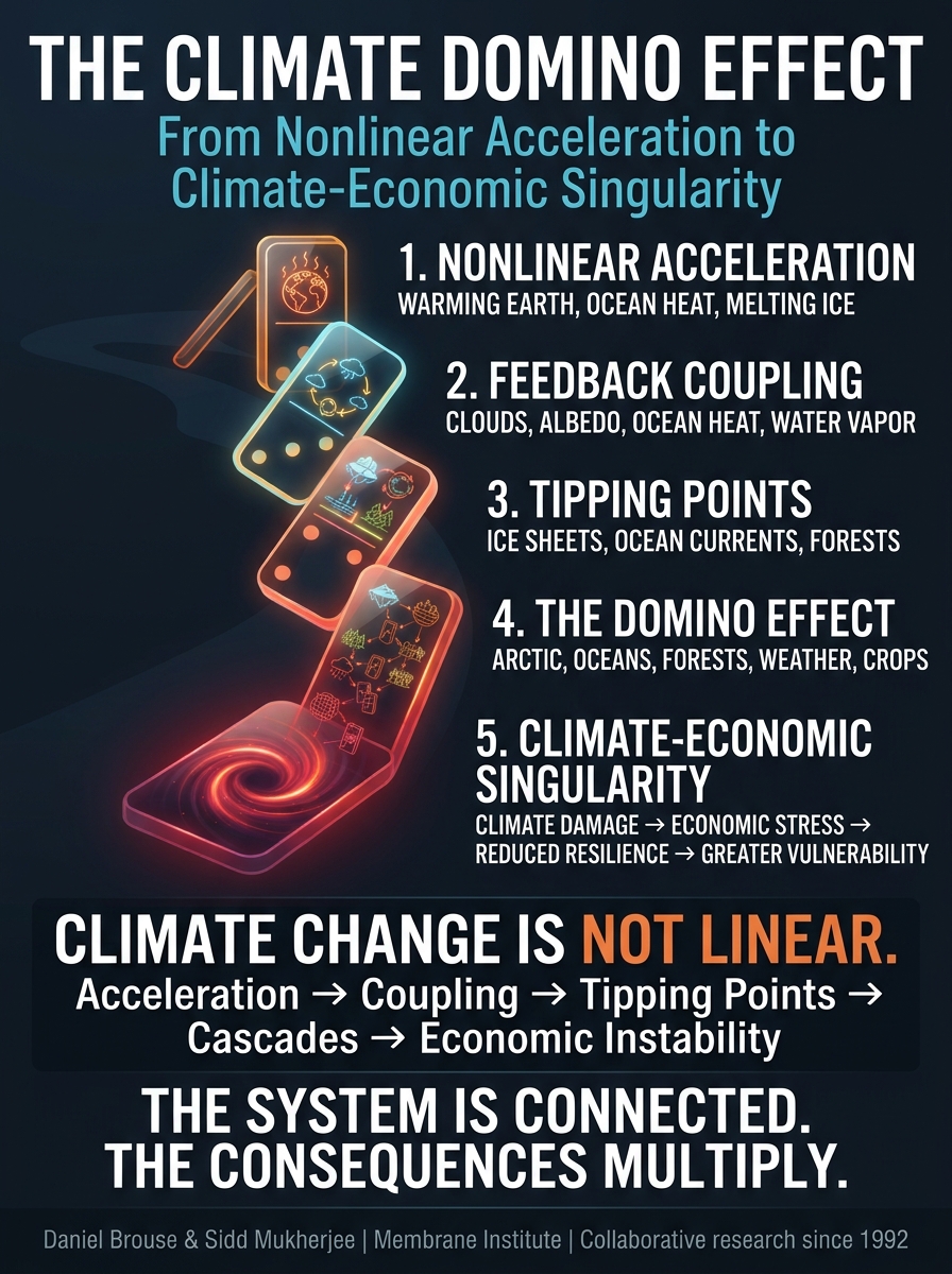
Five interconnected concepts form the foundation of this framework:

  1. Nonlinear Acceleration Hypothesis: Climate impacts increase at changing rates, with the possibility that acceleration itself is increasing.
  2. Feedback Coupling: Individual climate feedback mechanisms interact, creating interconnected amplification networks.
  3. Climate Tipping Points: Critical thresholds alter the stability and behavior of individual Earth-system components.
  4. The Domino Effect: Destabilization in one component propagates through interconnected physical, biological, ecological, and socioeconomic systems.
  5. Climate-Economic Singularity: Climate and economic feedback systems increasingly interact, amplifying instability and undermining the capacity to recover from subsequent disturbances.

A central supporting contribution is the 2026 National Science Review paper, The Domino Effect of Climate Tipping Points: A Multidisciplinary Perspective on Global Risks. Its multidisciplinary treatment of interconnected tipping elements and cascading risks provides an important scientific foundation for understanding climate disruption as a network phenomenon rather than a collection of isolated environmental events.

This paper extends that perspective through the integration of nonlinear dynamics, climate feedback analysis, observational indicators, economic transmission mechanisms, and systemic risk.

The central argument is that climate disruption increasingly involves self-reinforcing interactions within the Earth system, while its consequences propagate into economic systems that depend on environmental stability. As these systems become more tightly coupled, historical linear assumptions, conventional risk assessments, and backward-looking climate baselines become progressively less reliable.

The defining challenge is no longer simply measuring how much the planet is warming. It is understanding how rapidly the interconnected systems supporting civilization are changing, how disturbances propagate between them, and whether economic and institutional resilience can keep pace.


1. Introduction: From Global Warming to Earth-System Destabilization

The conventional description of climate change emphasizes the relationship between greenhouse gas emissions, atmospheric concentrations, radiative forcing, and increasing global temperatures.

These relationships remain fundamental to understanding anthropogenic warming. However, they do not fully describe the increasingly complex interactions occurring throughout the Earth system.

The planet is not a collection of independent environmental components. Its atmosphere, oceans, cryosphere, land surface, biosphere, and geological systems exchange energy and matter through interconnected physical and biological processes.

Changes in one component alter the conditions experienced by others.

The resulting interactions can amplify initial disturbances, accelerate subsequent changes, and destabilize systems that previously absorbed environmental stress.

This is the central premise of our collaborative research.

Beginning with the Nonlinear Acceleration Hypothesis, our work has progressively examined the transition from individual climate feedbacks to interconnected feedback networks, tipping-point interactions, cascading disruption, and ultimately climate-economic coupling.

The progression can be summarized:

Warming
↓
Feedback Activation
↓
Feedback Coupling
↓
Nonlinear Acceleration
↓
Threshold Transitions
↓
Cascading Tipping Points
↓
Ecological and Economic Disruption
↓
Climate-Economic Amplification

These processes are not necessarily sequential. They overlap, interact, and develop at different rates.

Nevertheless, the progression provides an integrated framework for examining the changing behavior of the Earth system.

2. The Nonlinear Acceleration Hypothesis

2.1 Origins and development

The Nonlinear Acceleration Hypothesis was developed by Brouse and Mukherjee in the late 1990s.

The original proposition was that climate impacts would not increase in a simple linear relationship with time. Instead, interactions among climate processes would produce increasingly consequential changes through reinforcing feedback mechanisms.

The hypothesis was subsequently developed through investigations into:

  • Nonlinear climate dynamics.
  • Chaos theory and complex adaptive systems.
  • Thermal energy redistribution.
  • Climate feedback mechanisms.
  • Cryosphere and ocean interactions.
  • Ecosystem degradation.
  • Accelerating climate-related economic losses.

The central distinction is between the rate at which climate change occurs and the rate at which that rate changes.

A system can experience increasing impacts without necessarily experiencing increasing acceleration. Likewise, a system can accelerate at a constant rate without experiencing increasing acceleration.

Our framework examines the higher-order dynamics.

2.2 First, second, and third derivatives

For a climate-impact indicator represented by I(t):

First derivative:

dI/dt = Rate of change.

Second derivative:

d²I/dt² = Acceleration.

Third derivative:

d³I/dt³ = Climate Jerk.

Climate Jerk describes the rate of change in acceleration.

When the third derivative is positive over an appropriately defined interval, acceleration is increasing.

This provides an additional dimension for investigating climate behavior beyond conventional trend analysis.

A positive third derivative does not establish that every climate indicator is accelerating, nor does it independently demonstrate that a tipping point has been crossed. The result depends on the indicator, measurement period, statistical treatment, and observational uncertainty.

Nevertheless, examining third-derivative behavior across multiple independent climate indicators offers a way to investigate whether the Earth system is entering a regime characterized by increasingly rapid changes.

2.3 Time compression

One of the most consequential implications of nonlinear acceleration is time compression.

Climate changes historically associated with longer timescales can produce increasingly rapid consequences as multiple processes interact.

Our research examines the compression of characteristic doubling times across climate-impact indicators, including extreme precipitation, heat extremes, wildfire behavior, ice loss, and economic damage.

The purpose is not to assume that every climate variable follows a single exponential trajectory. Different indicators have different physical constraints, statistical distributions, and response times.

Rather, the observed and proposed compression of characteristic timescales provides a framework for investigating whether climate disruption is becoming increasingly concentrated within shorter periods.

2.4 The failure of historical climate baselines

The traditional 30-year climate normal is useful for describing long-term climate conditions. However, rapidly changing climate distributions create an important limitation.

If temperatures, precipitation extremes, atmospheric moisture, and seasonal patterns change substantially within a decade, a 30-year average can increasingly describe conditions that no longer represent the current climate.

The faster the climate changes, the more a backward-looking baseline can lag behind actual conditions.

This has direct consequences for:

  • Weather forecasting.
  • Infrastructure engineering.
  • Agricultural planning.
  • Insurance underwriting.
  • Property valuation.
  • Municipal budgeting.
  • Financial risk assessment.

Our April 2026 paper, Climate Change Change: Third Derivatives, Time Compression, and the Collapse of the 30-Year Climate Baseline, develops this argument.

The central point is that institutions must increasingly evaluate the rate at which climate conditions change rather than relying exclusively on historical averages.

3. Feedback Coupling: From Individual Mechanisms to Interconnected Networks

3.1 The amplification mechanism

Climate feedbacks are processes through which an initial change produces an additional response. Positive feedbacks reinforce the original disturbance. Negative feedbacks counteract it.

The critical issue is that feedback mechanisms do not operate independently. They interact through shared energy flows, atmospheric circulation, ocean dynamics, biological processes, and changes in surface conditions.

Consequently, the combined behavior of interacting feedbacks can differ substantially from the behavior of individual mechanisms considered separately.

3.2 Major climate feedback mechanisms

Ice-albedo feedback

Declining snow and ice expose darker surfaces that absorb more incoming solar radiation. Additional energy absorption contributes to further warming and ice loss.

Ocean-cryosphere coupling

Increasing ocean heat contributes to basal ice-shelf melting, grounding-line retreat, and destabilization of marine-based ice sheets.

Water-vapor feedback

Warmer atmospheric conditions increase the capacity of the atmosphere to hold moisture. Increased water vapor amplifies the greenhouse effect.

Cloud feedback

Changes in cloud coverage, altitude, optical properties, and composition alter the balance between incoming solar radiation and outgoing terrestrial radiation.

Low-level cloud reductions are particularly important because these clouds reflect substantial incoming solar energy.

Biosphere-carbon feedback

Heat, drought, wildfire, pests, and atmospheric pollutants stress vegetation, reduce photosynthetic activity, and weaken natural carbon sinks.

Permafrost feedback

Thawing permafrost releases previously frozen organic carbon through microbial decomposition, increasing atmospheric carbon dioxide and methane.

These mechanisms create multiple pathways through which disturbances propagate throughout the Earth system.

3.3 The Coupled Climate Feedback Index

Our Coupled Climate Feedback Index provides an analytical framework for investigating interactions among major climate indicators.

The framework incorporates:

  • Cloud cover.
  • Surface albedo.
  • Sea ice.
  • Ocean heat content.
  • Global surface temperature.
  • Atmospheric water vapor.

The analysis includes directional normalization, trend treatment, and pairwise and higher-order relationships.

Particular attention is given to the interaction among surface albedo, ocean heat content, and cloud behavior.

The proposed weighting framework identifies the following relationships:

Feedback interactionProposed relative weight
Albedo × Ocean Heat Content14.3%
Cloud × Ocean Heat Content13.2%
Albedo × Cloud12.1%
Combined three-variable interaction39.6%

These figures represent the proposed analytical weighting structure, not independently established percentages of global warming or causal attribution.

The purpose of the index is to investigate whether relationships among climate indicators are changing in ways consistent with increasing feedback coupling.

3.4 Feedback networks

Individual feedback loops can become components of larger networks.

For example:

Ocean Heat Accumulation
↓
Sea-Ice and Ice-Shelf Loss
↓
Reduced Surface Albedo and Increased Ocean Exposure
↓
Additional Solar Energy Absorption
↓
Further Ocean Warming
↓
Additional Cryosphere Destabilization

A second pathway involves the biosphere:

Increasing Heat and Drought
↓
Vegetation Stress and Wildfires
↓
Reduced Photosynthesis and Carbon Uptake
↓
Weakened Carbon Sinks
↓
Higher Atmospheric Greenhouse Gas Concentrations
↓
Additional Warming

The interaction between these pathways creates opportunities for cross-system amplification.

This is the distinction between individual feedbacks and feedback coupling.

Our research into emerging feedback networks examines how these relationships develop into interconnected systems capable of transmitting disturbances across multiple Earth-system components.

4. Climate Tipping Points: Thresholds and Loss of Resilience

4.1 Critical transitions

A climate tipping point occurs when an Earth-system component crosses a critical threshold beyond which a relatively small additional disturbance can produce a major transition.

Such transitions are associated with nonlinear dynamics, bifurcation theory, hysteresis, and changes in system stability.

Before a tipping point, a system may absorb disturbances and return toward its previous condition. As resilience declines, recovery can become slower or less complete. After a critical transition, the system may move toward a different state even if the original forcing is subsequently reduced.

This distinction is particularly important when evaluating the difference between preventing further destabilization and restoring an earlier environmental condition.

4.2 Major tipping elements

Cryosphere

  • Greenland Ice Sheet destabilization.
  • West Antarctic Ice Sheet destabilization.
  • Antarctic marine ice-sheet instability.
  • Arctic sea-ice loss.
  • Mountain glacier retreat.
  • Permafrost degradation.

Ocean and marine systems

  • Atlantic Meridional Overturning Circulation (AMOC) weakening.
  • Changes in ocean overturning and regional circulation.
  • Marine ecosystem transitions.
  • Ocean deoxygenation.
  • Coral reef ecosystem degradation.
  • Disruption of marine biological carbon pumps.

Terrestrial ecosystems

  • Amazon rainforest dieback.
  • Boreal forest transitions.
  • Large-scale ecosystem degradation.
  • Loss of biodiversity and ecological resilience.

These systems are connected through heat redistribution, atmospheric circulation, ocean circulation, freshwater inputs, carbon exchange, and biological dependencies.

A disturbance in one system can therefore alter the stability of another.

4.3 Tipping points are not isolated events

The most important implication is that the stability of an individual tipping element cannot be evaluated entirely independently of its surrounding network.

The vulnerability of one system can increase as connected systems change.

For example, ocean warming affects ice shelves. Ice loss alters surface reflectivity and freshwater inputs. Freshwater changes can influence ocean circulation. Circulation changes can redistribute heat and nutrients, affecting marine ecosystems.

This creates a network of interacting vulnerabilities.

5. The Domino Effect: Cascading Tipping-Point Networks

5.1 The multidisciplinary perspective

The 2026 paper by Jun Meng and Deliang Chen, The Domino Effect of Climate Tipping Points: A Multidisciplinary Perspective on Global Risks, provides important supporting documentation for this framework. Published in National Science Review, the paper examines the broader consequences of interconnected tipping points and the potential for cascading transitions across multiple systems.

Its multidisciplinary perspective reinforces an important principle:

Climate tipping points are not simply individual thresholds. They are components of an interconnected network.

The use of network-based approaches, including multilayer connectivity and percolation concepts, provides a framework for investigating how local disturbances can propagate into larger systemic disruptions.

This complements our earlier work on feedback loops, tipping points, and the Domino Effect.

5.2 From dominoes to network cascades

The traditional domino analogy suggests that one event triggers another in a linear sequence.

The actual Earth system is more complex. One disturbance can affect several interconnected systems simultaneously. Those systems can then influence multiple additional components.

The resulting network contains overlapping pathways, feedback loops, thresholds, and dependencies.

Example 1: Arctic warming and cascading climate disruption

Arctic Warming
↓
Sea-Ice Loss
↓
Reduced Surface Albedo and Increased Solar Energy Absorption
↓
Changes in Ocean-Atmosphere Heat Exchange
↓
Changes in Atmospheric and Ocean Circulation
↓
Regional Temperature and Precipitation Changes
↓
Ecosystem Stress and Destabilization
↓
Agricultural Disruption and Economic Losses

This is an illustrative pathway, not a claim that every link occurs in a fixed sequence or that Arctic sea-ice loss alone necessarily triggers all subsequent changes.

Example 2: Ocean circulation and marine ecosystem disruption

Ocean Circulation Changes
↓
Altered Ocean Temperature and Nutrient Distribution
↓
Marine Deoxygenation and Ecosystem Stress
↓
Coral Reef Degradation and Fisheries Disruption
↓
Reduced Marine Food Production
↓
Food Security and Livelihood Pressures
↓
Economic Disruption in Coastal Communities

This pathway demonstrates how physical ocean disturbances can propagate into biological, ecological, and economic systems.

Example 3: Forest degradation and carbon-sink failure

Increasing Heat and Drought
↓
Vegetation Stress and Wildfire
↓
Forest Degradation and Reduced Photosynthesis
↓
Declining Carbon Uptake
↓
Weakened Terrestrial Carbon Sinks
↓
Additional Atmospheric Greenhouse Gas Accumulation
↓
Further Climate Stress

The important feature is the reinforcing relationship between ecosystem degradation and climate change.

5.3 Percolation and interconnected risk

Percolation theory provides a mathematical framework for examining how disturbances spread through connected networks. As network connectivity or interaction strength increases, localized disruptions can propagate across larger portions of a system.

Applied to climate science, this raises an important question:

At what point do interactions among individual tipping elements become sufficiently strong that localized disturbances can generate widespread systemic transitions?

There is no single established planetary threshold answering this question. However, multilayer network analysis provides a useful framework for studying how physical, biological, ecological, and socioeconomic systems interact.

5.4 The importance of cascading effects

The Domino Effect changes the way climate risk must be evaluated.

A tipping element may appear geographically isolated, but its consequences can extend across the planet through atmospheric, oceanic, ecological, and economic connections.

The resulting risks cannot be adequately characterized by evaluating individual events in isolation.

The relevant question becomes how disturbances interact, how quickly they propagate, and whether the affected systems retain sufficient resilience to prevent additional transitions.

6. Climate-Economic Coupling: The Transmission of Physical Risk

6.1 The economy is embedded within the Earth system

The global economy depends on relatively stable environmental conditions. Agriculture requires productive soils, reliable water, and predictable growing conditions. Energy systems require functioning infrastructure and dependable resources. Transportation and international trade depend on ports, waterways, roads, railways, and shipping networks. Financial institutions depend on functioning businesses, insurable assets, reliable collateral, and stable economic activity.

These are not independent of environmental conditions.

The economy is embedded within the Earth system.

Consequently, environmental degradation creates economic consequences that extend far beyond the immediate cost of repairing physical damage.

6.2 Major economic transmission mechanisms

Agriculture and food security

Heat stress, drought, flooding, changing precipitation patterns, and ecosystem degradation affect crop production, livestock, fisheries, and food distribution.

Simultaneous disruptions across major agricultural regions increase the potential for global food-price instability.

Insurance and financial markets

Increasing losses, higher reconstruction costs, changing hazard exposure, and declining insurability affect property values, insurance availability, mortgage markets, and financial risk.

Insurance withdrawal transfers additional exposure to homeowners, businesses, municipalities, lenders, and governments.

Infrastructure and public finances

Flooding, extreme precipitation, coastal erosion, extreme heat, and severe storms increase maintenance and replacement costs.

Governments face competing demands for emergency response, reconstruction, adaptation, public services, and debt servicing.

Energy and transportation

Extreme temperatures, water shortages, flooding, and severe weather threaten electricity generation, transmission infrastructure, transportation networks, and industrial operations.

International trade and supply chains

Disruptions in agricultural production, shipping, ports, energy supplies, and manufacturing propagate through international markets. These transmission mechanisms create an additional layer of cascading risk.

A climate disturbance initiates an economic disturbance, which can then increase vulnerability to subsequent climate disturbances.

6.3 Economic damage becomes endogenous

Conventional economic analysis frequently treats environmental damage as an external cost. This becomes increasingly inadequate when climate disruption begins changing the operating conditions of the economy itself.

Consider the insurance and property market:

Increasing Property Losses
↓
Higher Insurance Premiums
↓
Reduced Property Affordability
↓
Insurance Withdrawal and Mortgage Constraints
↓
Declining Property Values
↓
Reduced Municipal Tax Revenues
↓
Constrained Infrastructure Investment
↓
Greater Exposure to Subsequent Climate Damage

The consequences extend beyond the original environmental event. Economic damage becomes an internal component of the climate-risk system.

This is the foundation of climate-economic coupling.

7. The Climate-Economic Singularity

7.1 Defining the singularity framework

The Climate-Economic Singularity is our proposed framework describing the convergence of nonlinear climate acceleration, reinforcing feedback networks, cascading tipping points, and increasingly interconnected economic instability.

The term singularity is used as a systems-level concept rather than a claim that a literal mathematical singularity or a single irreversible global economic collapse has been demonstrated.

In our March 2026 paper, Approaching Singularity: Third Derivatives, Nonlinear Collapse, and Coupled Climate-Economic Instability, we developed this concept through the examination of nonlinear dynamics, physical analogies, third-derivative behavior, and coupled climate-economic processes.

A singularity-like regime is characterized by:

  • Increasing sensitivity to relatively small disturbances.
  • Accelerating changes in system behavior.
  • Reinforcing feedback mechanisms.
  • Declining reliability of historical relationships.
  • Increasing difficulty predicting future trajectories.
  • Greater potential for abrupt transitions and cascading failures.

The essential distinction is that the system is no longer adequately described through isolated linear relationships.

7.2 The climate-economic feedback loop

The interaction can be represented as:

CLIMATE DISRUPTION
Increasing heat, extreme precipitation, drought, flooding, wildfire, ocean changes, and ecosystem degradation.

↓

ECONOMIC DAMAGE
Agricultural losses, infrastructure destruction, insurance claims, property devaluation, supply-chain disruptions, and rising public expenditures.

↓

FINANCIAL AND INSTITUTIONAL STRESS
Higher insurance costs, credit risk, municipal fiscal pressure, capital losses, market instability, and reduced investment capacity.

↓

REDUCED ADAPTIVE CAPACITY
Less available capital for infrastructure protection, climate adaptation, ecosystem restoration, and economic resilience.

↓

GREATER CLIMATE VULNERABILITY
More exposed infrastructure, vulnerable communities, fragile supply chains, and reduced capacity to absorb subsequent disturbances.

↓

ADDITIONAL ECONOMIC DAMAGE
The cycle reinforces itself.

This is the critical distinction between conventional climate-economic risk and the singularity framework.

Climate disruption does not simply impose an increasing financial cost. It can undermine the economic capacity required to manage subsequent climate damage.

7.3 Third-derivative behavior

Our singularity framework examines the possibility that both climate and economic indicators exhibit increasing rates of acceleration.

The progression is:

dI/dt > 0 — Impacts are increasing.

d²I/dt² > 0 — Impacts are accelerating.

d³I/dt³ > 0 — Acceleration itself is increasing.

These relationships must be evaluated against specific indicators, observation periods, and statistical methods.

The important question is whether multiple independent climate and economic indicators increasingly exhibit this behavior.

Our research examines ocean heat content, sea-level rise, ice-sheet mass loss, atmospheric circulation, extreme weather losses, and economic exposure as components of this broader investigation.

7.4 Ocean Solvency and the Ocean Maelstrom

A particularly important extension of the Climate-Economic Singularity framework is our November 10, 2026 update, Ocean Maelstrom: Navigating the Climate Storm.

The report examines the systemic economic implications of ocean degradation, incorporating the Ocean Solvency framework developed in the November 2026 report by the Institute and Faculty of Actuaries, the University of Exeter, and The Ocean Race.

Ocean Solvency describes the continuing capacity of the ocean to provide the ecosystem services upon which human societies and economies depend.

These services include:

  • Global climate regulation and heat redistribution.
  • Marine food production and biodiversity.
  • Oxygen production and carbon absorption.
  • Global water cycles and weather patterns.
  • International commerce and maritime transportation.
  • Economic productivity and financial stability.

The Ocean Maelstrom scenario illustrates how multiple interacting ocean, climate, ecological, and geopolitical pressures can propagate through economic systems.

The sequence can be represented as:

Ocean Degradation
↓
Climate Disruption
↓
Food and Agricultural Instability
↓
Inflation and Supply-Chain Disruption
↓
Economic Contraction
↓
Financial and Sovereign Instability
↓
Reduced Adaptive Capacity
↓
Greater Vulnerability to Subsequent Disruptions

The scenario also examines exposure involving insurance markets, pension funds, investment portfolios, government finances, and retirement security.

Importantly, the scenario is a systemic-risk assessment, not a prediction of a specific economic contraction. Its significance is that ocean degradation can affect multiple components of economic stability simultaneously.

The ocean is not separate from the economy. It is foundational economic infrastructure.

7.5 From climate damage to economic amplification

The Climate-Economic Singularity framework extends the Domino Effect beyond the physical and ecological environment.

The interconnected system now includes:

  • Climate feedback networks.
  • Ecological and biological systems.
  • Agricultural and food systems.
  • Insurance and property markets.
  • Banking and financial institutions.
  • Infrastructure and energy networks.
  • Government budgets and sovereign finances.
  • International trade and supply chains.

As these systems become more tightly coupled, disruptions can propagate across multiple sectors. The resulting consequences can exceed the sum of individual losses.

This is the transition from environmental risk to systemic economic risk.

8. Integrating the Five Concepts: One Unified Framework

The five concepts developed throughout our research describe interconnected dimensions of the same evolving process.

ConceptPrincipal mechanismSystemic consequence
Nonlinear Acceleration HypothesisIncreasing rates of climate change and accelerationHistorical trends become inadequate
Feedback CouplingReinforcement among interacting climate processesGreater amplification of disturbances
Climate Tipping PointsCritical thresholds and changes in system stabilityAbrupt and potentially irreversible transitions
Domino EffectPropagation across interconnected systemsCascading environmental and ecological disruption
Climate-Economic SingularityCoupling of climate and economic feedback systemsSystemic economic instability and declining resilience

The complete framework can be summarized:

WARMING
↓
FEEDBACK ACTIVATION
↓
FEEDBACK COUPLING
↓
NONLINEAR ACCELERATION
↓
THRESHOLD TRANSITIONS
↓
CASCADING TIPPING POINTS
↓
ECOLOGICAL AND ECONOMIC DISRUPTION
↓
CLIMATE-ECONOMIC AMPLIFICATION
↓
REDUCED SYSTEMIC RESILIENCE

This is a conceptual progression, not a fixed sequence of inevitable events. Individual processes can overlap, reinforce one another, and develop at different rates.

Nevertheless, the integrated framework provides a means of examining the transition from emissions-driven warming to increasingly interconnected Earth-system and economic instability.

9. Measuring and Monitoring an Interconnected System

9.1 Beyond global average temperature

Global average temperature remains an essential climate indicator, but it cannot independently characterize the stability of the entire Earth system.

A more comprehensive approach must examine:

  • Earth’s energy imbalance.
  • Ocean heat content.
  • Sea-ice extent and thickness.
  • Surface albedo.
  • Cloud properties.
  • Atmospheric water vapor.
  • Ocean circulation.
  • Ice-sheet mass and grounding-line behavior.
  • Ecosystem productivity.
  • Atmospheric and terrestrial carbon exchange.
  • Extreme precipitation and drought.
  • Agricultural productivity.
  • Climate-related economic losses.

The relationships among these indicators are as important as their individual trends.

9.2 Early-warning indicators

Systems approaching critical transitions can exhibit changes in their behavior before a major transition occurs.

Potential warning signals include:

  • Increasing variance.
  • Increasing autocorrelation.
  • Critical slowing down.
  • Changes in spatial correlations.
  • Increasing sensitivity to disturbances.
  • Altered recovery rates following perturbations.

These indicators can provide useful information about changing resilience. However, early-warning signals are not universal, and their absence does not establish that a system is stable.

The observational challenge is to identify changes in system behavior while distinguishing genuine shifts from natural variability, measurement limitations, and statistical artifacts.

9.3 Integrating physical and economic observations

The next generation of climate-risk analysis must connect Earth-system observations with economic and financial indicators.

A comprehensive monitoring framework integrates:

  1. Physical climate observations.
  2. Nonlinear dynamical analysis.
  3. Climate feedback networks.
  4. Multilayer tipping-point analysis.
  5. Ecological and biogeochemical measurements.
  6. Agricultural and infrastructure exposure.
  7. Insurance and financial risk indicators.
  8. Government fiscal exposure.
  9. AI-assisted pattern recognition and early-warning systems.

This approach improves the ability to identify not only individual climate thresholds but also the interactions that increase the potential for cascading disruptions.

It also provides a more realistic assessment of how environmental changes propagate through the global economy.

10. Implications for Climate Policy and Economic Risk Management

The integrated framework has important implications for climate policy.

Emissions reductions remain essential because they limit additional external forcing and reduce the likelihood of further destabilization. However, climate policy must also address the internal dynamics of the Earth system and the growing economic consequences of interconnected climate disruption.

Five priorities

1. Protect climate-regulating systems

Prioritize the cryosphere, forests, wetlands, marine ecosystems, and other systems that contribute to planetary climate regulation.

2. Monitor coupled feedbacks

Develop integrated observational systems that identify changes in relationships among ocean heat, albedo, clouds, ice, atmospheric moisture, and biological carbon uptake.

3. Evaluate cascading risk

Assess infrastructure, food production, water security, insurance markets, and financial institutions against compound and interconnected climate hazards rather than isolated historical events.

4. Build economic resilience

Strengthen infrastructure, diversify supply chains, improve emergency preparedness, protect natural systems, and reduce financial exposure to correlated climate risks.

5. Integrate mitigation with measurable environmental benefits

Climate stewardship must extend beyond reducing emissions to include actions that improve the functioning of natural systems and reduce environmental stress.

Our Integrated Climate Stewardship framework expresses this through a straightforward principle:

ZERO-OUT + BENEFIT-IN.

Reduce environmental damage while actively contributing measurable benefits to the systems that sustain life and economic activity.

The objective is not merely to slow deterioration. It is to restore and strengthen resilience wherever possible.


11. Conclusion: The Transition to Systemic Climate-Economic Instability

The most important implication of our collaborative research is that climate change cannot be adequately evaluated as a linear response to greenhouse gas emissions.

The Earth system is interconnected, nonlinear, and capable of abrupt transitions.

The Nonlinear Acceleration Hypothesis identifies the increasing importance of acceleration in climate disruption.

Feedback Coupling explains how individual amplification mechanisms interact and form larger networks.

Climate Tipping Points identify critical thresholds beyond which major Earth-system transitions can occur.

The Domino Effect explains how those transitions propagate through interconnected physical, biological, ecological, and socioeconomic networks.

The Climate-Economic Singularity extends the analysis into the global economy, where climate damage increasingly affects the systems responsible for maintaining economic stability and financing recovery.

The 2026 analysis by Meng and Chen provides an important multidisciplinary foundation for understanding how tipping elements interact and how localized disturbances can generate cascading global risks.

Our collaborative work extends this perspective by integrating nonlinear acceleration, climate feedback coupling, third-derivative analysis, and economic transmission mechanisms into a unified framework.

The resulting picture is one of increasing interdependence.

Climate instability damages economic systems. Economic instability reduces the resources available for adaptation and resilience. Reduced resilience increases exposure to subsequent climate disturbances.

The cycle reinforces itself.

The consequences extend from the physical environment into property markets, insurance systems, agriculture, infrastructure, financial institutions, government budgets, and international commerce.

The global economy is operating within an Earth system whose stability it depends upon but whose destabilization it must increasingly absorb.

This creates a fundamental challenge for conventional economic analysis: the systems supporting economic production and financial stability are themselves exposed to the environmental deterioration driving the risks.

The central question is no longer simply how much additional warming the planet will experience. It is how rapidly the interconnected systems supporting civilization are losing resilience, how disturbances propagate between them, and whether economic institutions can adapt at a rate sufficient to keep pace.

Understanding this transition is essential to anticipating the next phase of climate risk.

The solution requires more than measuring change. It requires understanding the interactions driving change, recognizing the thresholds that alter system behavior, and protecting the environmental and economic foundations of civilization.


References and Supporting Research

A. Principal collaborative research by Brouse and Mukherjee

1. Nonlinear Acceleration of Climate Change (1999)

Brouse, D., & Mukherjee, S. (1999). Nonlinear Acceleration of Climate Change. Membrane Institute Working Paper Series.

Foundational development of the Nonlinear Acceleration Hypothesis.

2. Tipped Tipping Points and the Domino Effect: Accelerating Climate Collapse (2026)

Brouse, D., & Mukherjee, S. The Human Induced Climate Change Experiment and the Domino Effect.

https://kingarthur.com/global_warming/Climate-Science-Resources.html#Climate-Change-Change

Develops the relationship among nonlinear acceleration, tipping-point interactions, feedback networks, and cascading climate disruption.

3. Climate Change Change: Third Derivatives, Time Compression, and the Collapse of the 30-Year Climate Baseline (April 2026)

Brouse, D., & Mukherjee, S. (2026).

https://kingarthur.com/global_warming/Climate-Change-Change.html

Examines third-derivative behavior, climate time compression, changing climate baselines, and implications for forecasting and economic risk.

4. Approaching Singularity: Third Derivatives, Nonlinear Collapse, and Coupled Climate-Economic Instability (March 2026)

Brouse, D., & Mukherjee, S. (2026).

https://kingarthur.com/global_warming/Singularity-Climate-Economic-Coupling.html

Develops the Climate-Economic Singularity framework through nonlinear dynamics, third derivatives, physical analogies, and interconnected climate-economic feedback systems.

5. Climate Jerk Surge: Albedo-Cloud-Ocean Heat Content Triad (September 2026)

Brouse, D. (2026).

Available through the Singularity research collection:

https://kingarthur.com/global_warming/Climate-Science-Resources.html#Singularity

Examines the interaction among surface albedo, cloud behavior, and ocean heat content.

6. Climate Jerk Surge Math and Methods (September 2026)

Brouse, D. (2026).

Available through the Singularity research collection:

https://kingarthur.com/global_warming/Climate-Science-Resources.html#Singularity

Documents the analytical methods associated with the Coupled Climate Feedback Index and higher-order feedback interactions.

7. Observational Evidence for Climate Jerk: Multidisciplinary Indicators of Accelerating Climate Acceleration (June 2026)

Brouse, D., & Mukherjee, S. (2026).

Available through the Singularity research collection:

https://kingarthur.com/global_warming/Climate-Science-Resources.html#Singularity

Examines multiple observational indicators and their implications for third-derivative climate behavior.

8. The Compression of Doubling Times Across Earth-System Indicators: Evidence for Increasing Nonlinearity in the Climate System (June 2026)

Brouse, D., & Mukherjee, S. (2026).

Available through the Singularity research collection:

https://kingarthur.com/global_warming/Climate-Science-Resources.html#Singularity

Examines changing characteristic timescales across multiple Earth-system indicators.

9. Emergent Climate Dynamics: The Nonlinear Acceleration of Climate Impacts (March 2026)

Brouse, D., & Mukherjee, S. (2026).

Available through the Singularity research collection:

https://kingarthur.com/global_warming/Climate-Science-Resources.html#Singularity

Develops the nonlinear dynamics framework underlying accelerating climate impacts.

10. A Unified Energetics Framework for Accelerating Climate Change: From Radiative Forcing to Drag Physics (March 2026)

Brouse, D., & Mukherjee, S. (2026).

Available through the Singularity research collection:

https://kingarthur.com/global_warming/Climate-Science-Resources.html#Singularity

Examines climate acceleration through an integrated energy and physical-dynamics framework.

11. The Compression of Time: Third Derivatives, Vortex Dynamics, and Wormholes in Climate-Economic Singularity (March 2026)

Brouse, D., & Mukherjee, S. (2026).

Available through the Singularity research collection:

https://kingarthur.com/global_warming/Climate-Science-Resources.html#Singularity

Explores time compression, nonlinear amplification, and singularity-like system behavior.

12. Ocean Maelstrom: Navigating the Climate Storm (November 10, 2026)

Brouse, D., & Mukherjee, S. (2026). Climate-Economic Coupling and Singularity: Ocean Solvency and the Ocean Maelstrom.

https://kingarthur.com/global_warming/Singularity-Climate-Economic-Coupling.html

Examines the transmission of ocean degradation through food security, supply chains, insurance, pensions, financial markets, and economic stability.

B. External scientific supporting research

13. The Domino Effect of Climate Tipping Points: A Multidisciplinary Perspective on Global Risks (2026)

Meng, J., & Chen, D. (2026). National Science Review, 13(20), nwag042.

https://academic.oup.com/nsr/article/13/20/nwag042/8437927

Primary external supporting paper for interconnected tipping elements, multilayer networks, and cascading global risks.

14. Tipping Elements in the Earth’s Climate System (2008)

Lenton, T. M., et al. (2008). Proceedings of the National Academy of Sciences, 105(6), 1786–1793.

https://doi.org/10.1073/pnas.0705414105

15. Trajectories of the Earth System in the Anthropocene (2018)

Steffen, W., et al. (2018). Proceedings of the National Academy of Sciences, 115(33), 8252–8259.

https://doi.org/10.1073/pnas.1810141115

16. Early-Warning Signals for Critical Transitions (2009)

Scheffer, M., et al. (2009). Nature, 461, 53–59.

https://doi.org/10.1038/nature08227

17. Catastrophic Cascade of Failures in Interdependent Networks (2010)

Buldyrev, S. V., et al. (2010). Nature, 464, 1025–1028.

https://doi.org/10.1038/nature08932

18. Climate Tipping Point Interactions and Cascades: A Review (2024)

Wunderling, N., et al. (2024). Earth System Dynamics, 15, 41–74.

https://doi.org/10.5194/esd-15-41-2024

19. Physics-Based Early Warning Signal Shows That AMOC Is on Tipping Course (2024)

van Westen, R. M., Kliphuis, M., & Dijkstra, H. A. (2024). Science Advances, 10, eadk1189.

https://doi.org/10.1126/sciadv.adk1189


Authors and Research Affiliations

Daniel Brouse
Independent Climate Researcher and Economist
Co-founder, Membrane Institute
Research interests: Nonlinear climate dynamics, climate-economic coupling, financial risk, climate feedback networks, and integrated climate stewardship.

Sidd Mukherjee, Ph.D.
Independent Physicist
Co-founder, Membrane Institute
Research interests: Physics, nonlinear systems, energy dynamics, mathematical modeling, and climate-system interactions.

Membrane Institute / Membrane.com
Collaborative independent research initiated in 1992.

This paper synthesizes the authors’ collaborative research and extends it through an integrated Earth-system and climate-economic risk framework. The proposed indices, acceleration metrics, and singularity framework are research constructs whose quantitative interpretations should be evaluated against observational evidence, statistical uncertainty, and established physical models.
bookmark_borderClimate-Economic Coupling

Simplified Overview

🌊 OCEAN MAELSTROM: THE CLIMATE-ECONOMIC SINGULARITY IS COMING INTO FOCUS

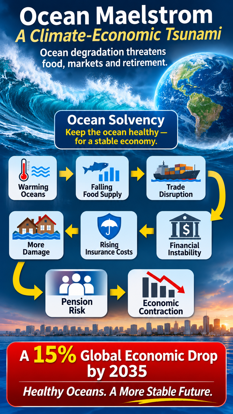
A landmark November 10, 2026 report from the Institute and Faculty of Actuaries, the University of Exeter, and The Ocean Race connects the dots between accelerating ocean degradation and global economic instability.

Its message is profound: The climate crisis is no longer just an environmental problem. It is becoming a systemic economic and financial crisis.

The report introduces Ocean Solvency—the ocean’s ability to continue providing the essential services upon which global civilization and economic activity depend.

But the implications go much further.

🌡️ Ocean degradation and climate disruption
→ Declining food production and rising prices
→ International trade and supply-chain disruptions
→ Increasing insurance losses
→ Financial market instability
→ Pension and retirement risks
→ Economic contraction.

Implications for Climate-Economic Coupling and Singularity

This is precisely the kind of interconnected, nonlinear risk that underlies the climate-economic coupling and singularity framework we’ve been developing.

Climate impacts do not occur in isolation. They propagate through interconnected physical, ecological, geopolitical, and financial systems. Each disruption creates additional pressures, while weakening the capacity of other systems to absorb the next shock.

The feedback becomes economic as well as environmental.

As climate disruption accelerates, economic losses increase. As economic stability deteriorates, the resources available for adaptation and resilience decline. That creates another reinforcing feedback loop.

The report explores a modeled scenario in which ocean-related shocks contribute to a 15% reduction in global economic output by 2035. This is a systemic-risk scenario.

The fundamental economic reality is difficult to escape:

The global economy cannot remain solvent while the natural systems supporting it become insolvent.

The climate-economic singularity is about more than rising temperatures. It is about the accelerating coupling of systems, the amplification of cascading failures, and the growing difficulty of containing consequences once multiple thresholds are crossed.

🌎 The ocean is not separate from the economy. It is part of the infrastructure that makes the global economy possible.

Read the report:

https://www.kingarthur.com/global_warming/Singularity-Climate-Economic-Coupling.html#Ocean-Maelsrtom

#OceanMaelstrom #OceanSolvency #ClimateEconomicCoupling #ClimateSingularity #SystemicRisk #ClimateEconomics #ClimateChange #FinancialStability

Update: Ocean Maelstrom — The Emerging Climate-Economic Feedback System

November 12, 2026

By Daniel Brouse and Sidd Mukherjee

5.5 Ocean Solvency and the Ocean Maelstrom: A New Dimension of Systemic Risk

Published November 10, 2026, Ocean Maelstrom: Navigating the Climate Storm is a landmark systemic-risk report developed by the Institute and Faculty of Actuaries (IFoA), the University of Exeter, and The Ocean Race.

The report provides an important independent assessment of the increasingly interconnected risks linking ocean degradation, climate instability, and global economic systems. Its central warning is that accelerating ocean degradation is not simply an environmental problem. It represents a growing threat to global food security, supply chains, insurance markets, pensions, financial markets, and overall economic stability.

Ocean Solvency: The Foundation of Economic Stability

The report introduces the concept of Ocean Solvency, defined by the ocean’s continuing ability to provide the essential ecosystem services upon which human societies and economies depend.

The ocean is fundamental to:

  • Global climate regulation and heat redistribution.
  • Food production and marine biodiversity.
  • Oxygen production and carbon absorption.
  • Global water cycles and weather patterns.
  • International commerce and maritime transportation.
  • Economic productivity and financial stability.

The report assesses current Ocean Solvency risk as severe, with the potential to become catastrophic to extreme by 2050 under a business-as-usual trajectory.

This introduces an important economic distinction: financial systems cannot remain solvent indefinitely if the natural systems supporting economic production become insolvent.

Ocean Maelstrom: A Systemic Risk Scenario

The report develops an Ocean Maelstrom scenario to demonstrate how multiple interacting pressures can produce cascading economic consequences.

Importantly, this is a plausible systemic-risk scenario, not a forecast. It examines how six individually plausible ocean, climate, and geopolitical pressures could interact between 2027 and 2035, producing consequences substantially greater than the sum of their individual impacts.

The scenario illustrates the transmission of physical climate and ecological disruptions through interconnected systems:

  1. Ocean and climate disruption: Marine heatwaves, ocean circulation changes, declining biodiversity, and deteriorating marine ecosystems undermine ocean productivity and climate regulation.
  2. Food and agricultural disruption: Changes in ocean conditions, fisheries, rainfall patterns, and agricultural production reduce food availability and increase food prices.
  3. Supply-chain and trade disruption: Disruptions to marine resources, maritime infrastructure, ports, and international commerce amplify economic instability.
  4. Insurance and infrastructure exposure: Increasing coastal damage, flooding, property losses, and infrastructure risks intensify insurance pressures and undermine asset valuations.
  5. Sovereign and financial instability: Economic contraction, inflation, declining revenues, and increased government expenditures create additional pressure on national finances and financial markets.
  6. Pension and retirement exposure: Investment losses, inflation, declining purchasing power, and weakened economic growth threaten long-term retirement security.

The Financial Consequences

One of the report’s most significant findings concerns the exposure of global retirement systems.

Global pension funds hold approximately $68.3 trillion in assets. Under the Ocean Maelstrom scenario, ocean-related shocks contribute to a modeled 15% reduction in global economic output by 2035.

This is not a prediction of a 15% economic contraction. It is a scenario-based assessment demonstrating the magnitude of potential systemic exposure.

The consequences extend beyond investment portfolios. Inflation reduces purchasing power, economic contraction weakens pension contributions, and deteriorating corporate and sovereign finances threaten the underlying assets supporting retirement systems.

The report identifies a particularly important problem with conventional financial risk models: ocean-related risks can simultaneously affect investment assets, liabilities, contribution capacity, and inflation. These risks are interconnected, persistent, and potentially difficult to diversify away.

Implications for Climate-Economic Coupling and Singularity

The Ocean Maelstrom report provides an important extension of the climate-economic coupling framework presented in this analysis.

It demonstrates how environmental degradation propagates through interconnected physical, ecological, geopolitical, and economic systems. More importantly, it illustrates how these interactions generate reinforcing feedback loops that reduce the capacity of societies and financial institutions to absorb subsequent disruptions.

The resulting feedback sequence can be expressed as:

Ocean degradation → Climate disruption → Food insecurity → Inflation → Economic contraction → Financial instability → Reduced adaptive capacity → Greater vulnerability

This is not simply a linear chain of economic consequences. The individual components interact, reinforce one another, and create opportunities for cascading failures.

The relationship is particularly important when considered alongside the third-derivative framework developed in this paper:

dI/dt > 0

d²I/dt² > 0

d³I/dt³ > 0

The significance is that climate impacts increase, their rate of increase accelerates, and the acceleration itself increases. As physical and economic systems become more tightly coupled, disruptions can propagate faster and produce increasingly disproportionate consequences.

The Ocean Is Not Separate From the Economy

Traditional economic models frequently treat environmental degradation as an external cost. Ocean Maelstrom challenges that assumption by demonstrating that the ocean is foundational economic infrastructure.

The economic system is not independent of the Earth system. It is embedded within it.

When natural capital deteriorates, the resulting losses do not disappear simply because they are excluded from conventional accounting. They reappear as food-price inflation, insurance losses, infrastructure damage, declining productivity, financial instability, and increased public expenditures.

This creates an additional dimension of systemic risk: the deterioration of the natural systems that support economic activity simultaneously weakens the financial resources available to respond to that deterioration.

Conclusion: An Expanding Climate-Economic Singularity

Ocean Maelstrom reinforces the central argument of this analysis: climate instability and economic instability are increasingly interconnected components of a larger nonlinear system.

The report’s contribution is particularly significant because it translates ocean degradation into recognizable financial and actuarial risks. Food security, insurance, sovereign finances, investment portfolios, and retirement security are not separate issues. They are interconnected consequences of the same underlying Earth-system disruption.

The emergence of Ocean Solvency as a financial risk framework represents an important recognition that economic stability ultimately depends on environmental stability.

The climate-economic singularity is therefore not confined to rising temperatures, accelerating sea-level rise, or increasing disaster losses. It encompasses the progressive destabilization of the interconnected systems upon which global civilization depends.

The ocean is not merely another economic resource. It is part of the infrastructure that makes the global economy possible.


Primary Source

Trust, S., Ranchin, A., Hunt, L., Joslin, S., Chapman, G., & Abrams, J. F. (2026). Ocean Maelstrom: Navigating the Climate Storm. Institute and Faculty of Actuaries, University of Exeter, and The Ocean Race. November 2026.

https://actuaries.org.uk/media/mkefco0p/ocean-maelstrom-navigating-the-climate-storm_november-2026.pdf

bookmark_borderTrump Enabled Chinese Spy

Trump Was Warned About Nvidia CEO’s Relationship With Suspected Chinese Spy — Yet Invited Him Aboard Air Force One and to White House State Dinner

President Donald Trump says he believes Nvidia CEO Jensen Huang had no idea that the woman with whom he acknowledged having an intimate relationship was a suspected Chinese spy. Trump expressed confidence in Huang’s explanation, describing him as an “honorable guy.”

However, reporting by The New York Times raises significant questions about what Trump knew, when he knew it, and why he continued to give Huang access to some of the most sensitive diplomatic settings involving China.

1. The Air Force One Warning

According to The New York Times, Secretary of State Marco Rubio briefed Trump aboard Air Force One in May 2026, during the president’s trip to China.

Rubio reportedly informed Trump that U.S. intelligence had identified a relationship between Huang and Alice Huang, a Chinese businesswoman suspected of working with China’s Ministry of State Security.

The intelligence concerns were sufficiently serious that Rubio oversaw the preparation of a highly classified memorandum warning senior administration officials about the relationship.

Despite these warnings, Trump arranged for Jensen Huang to join his presidential delegation. During a stop in Alaska, Huang boarded Air Force One at Trump’s invitation and continued the journey to China.

The decision raises questions about how the administration evaluated the intelligence warning and whether national security concerns were adequately considered before granting Huang access to the presidential delegation.

2. The White House State Dinner

In September 2026, Trump hosted Chinese President Xi Jinping at a high-profile White House state dinner.

Despite the intelligence concerns surrounding Huang’s relationship with a suspected Chinese intelligence operative, Huang and his wife were invited to attend.

Huang was seated at the prominent head table alongside Trump and Xi.

The decision to include Huang in such a high-profile diplomatic setting raises additional questions about the administration’s handling of the intelligence concerns and its assessment of potential national security risks.

3. Trump’s Public Defense of Huang

Following the revelations, Trump defended Huang publicly.

Trump said Huang had told him he had no idea the woman was a spy and stated, “I really believe him.”

He also described Huang as an “honorable guy” and suggested that he should remain Nvidia’s CEO.

Meanwhile, Nvidia’s board has initiated an independent investigation into the relationship and associated national security concerns. The company has stated that it has no reason to believe its trade secrets or national security information were compromised, but that the investigation will examine the available evidence.

4. The Larger National Security Questions

This controversy extends beyond the personal relationship of a prominent technology executive.

Nvidia is a central supplier of advanced artificial intelligence chips, technologies that have major economic, military, and strategic implications in the competition between the United States and China.

The central questions are straightforward:

  • What intelligence did the administration possess about the suspected Chinese operation?
  • Why did Trump proceed with inviting Huang aboard Air Force One after receiving the reported warning?
  • Why was Huang subsequently seated alongside Trump and Xi at the White House state dinner?
  • Were appropriate national security safeguards maintained?
  • Did the administration adequately evaluate the potential risks to America’s technological and strategic interests?

These questions deserve serious congressional scrutiny and a transparent accounting of the administration’s decisions.

National security intelligence warnings are not simply political talking points. They exist to protect American interests. How those warnings are received, evaluated, and acted upon deserves accountability.

bookmark_border4.0% Inflation: Diesel Prices and the Coming Food Inflation

How Rising Energy Costs Move Through the Agricultural Supply Chain and Into Consumer Prices

By Daniel Brouse; Independent Economist, Financial Analyst, and Independent Climatologist

Simplified Overview

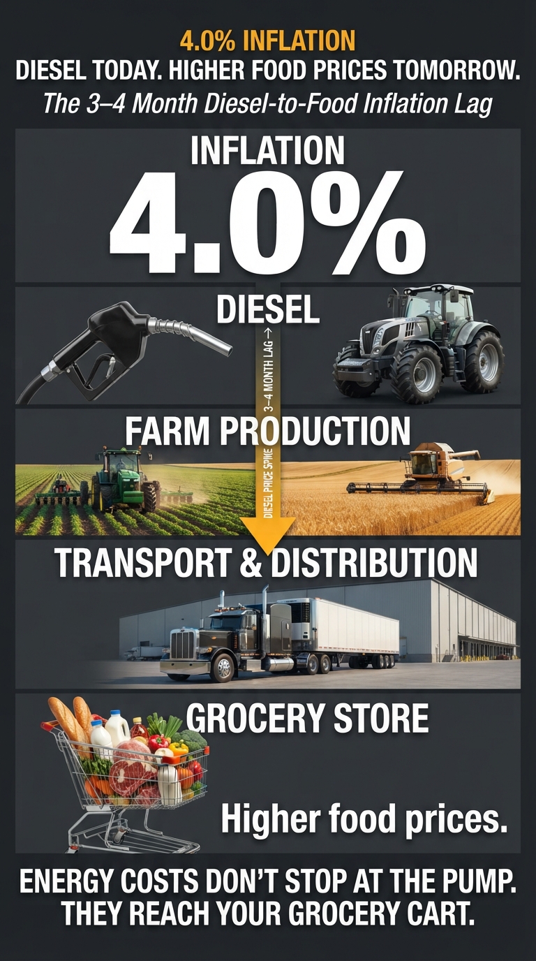
📈 4.0% INFLATION: DIESEL PRICES AND THE COMING FOOD INFLATION

With third-party calculations estimating annual consumer-price increases at 4.0%, up from 3.7% in September, monitoring diesel prices becomes particularly important when evaluating where food inflation is headed.

What you pay at the grocery store tomorrow may already be reflected in the diesel prices businesses are paying today.

Diesel is the lifeblood of the agricultural supply chain. It powers farm machinery, transports crops, moves food through processing facilities, and delivers products to grocery stores.

When diesel prices rise, the inflationary impact doesn’t stop at the fuel pump. It moves through the entire food supply chain, creating an estimated 3–4 month delay before higher operating costs work their way into consumer food prices.

🚜 Farm production
🚛 Freight and transportation
🏭 Food processing and distribution
🛒 Grocery-store prices

The economic lesson: Watch diesel prices today to understand food inflation tomorrow.

A closer look at the relationship between energy costs, agricultural production, and the inflationary pressures facing American households.

— Daniel Brouse

#Inflation #DieselPrices #FoodInflation #Economics #CPI #EnergyCosts #CostOfLiving

Introduction

Energy prices are a major driver of food inflation. Among the most important indicators is diesel fuel, which powers the machinery, transportation networks, and logistics infrastructure supporting the entire agricultural supply chain.

Diesel price increases can provide an early warning of broader food-price inflation, with an estimated transmission lag of approximately three to four months. This delay reflects the time required for higher fuel and operating costs to move through agricultural production, freight transportation, food processing, distribution, and retail pricing.

The relationship is particularly important because food inflation does not respond to energy-price increases instantaneously. Instead, rising costs accumulate throughout the supply chain, creating a delayed inflationary effect that eventually reaches consumers.

This process resembles a supply-chain bullwhip effect: an initial increase in fuel costs propagates through multiple stages of production and distribution, amplifying operating expenses before they appear in retail food prices.

1. The October 2026 Inflation Report

The October 2026 Consumer Price Index (CPI) report released by the U.S. Bureau of Labor Statistics showed that overall consumer prices increased 0.4% month-over-month, while core inflation, which excludes volatile food and energy prices, increased 0.3%.

Third-party inflation calculations estimate that overall U.S. consumer prices are running approximately 4.0% higher than a year ago, up from an estimated 3.7% in September.

Although the October annual comparison is not an official BLS twelve-month CPI calculation, the third-party estimate provides an additional perspective on the continuing inflationary pressures affecting American households.

The distinction matters because inflation is not simply a measurement of what consumers paid last month. It reflects the cumulative increase in the cost of living, including the essential expenses of food, transportation, housing, and energy.

The relationship between energy costs and food prices deserves particular attention because changes in fuel prices can affect agricultural production and distribution well before their full impact appears in consumer inflation statistics.

2. Why Diesel Prices Lead Food Inflation

Diesel is one of the fundamental inputs supporting the modern food economy. Its influence extends across four interconnected stages of the agricultural supply chain.

A. Agricultural Production: The Farm-Level Lag

Diesel powers much of the heavy equipment required to produce food, including:

  • Tractors and planting equipment.
  • Combines and harvesting machinery.
  • Irrigation pumps and agricultural transport vehicles.
  • Equipment used for moving crops and materials around farms.

The transmission mechanism:

When diesel prices increase, farmers face higher operating costs for planting, cultivating, irrigating, and harvesting crops.

Those expenses become embedded in production costs. Depending on the crop, growing season, and timing of the fuel purchase, the increased costs may not be reflected in food prices until the resulting harvest moves through processing and distribution.

The inflationary effect: Higher agricultural production costs eventually place upward pressure on wholesale and retail food prices.

B. Freight and Logistics: The Transportation Lag

Food is particularly dependent on transportation because it must move from farms to processors, warehouses, distributors, and grocery stores.

Diesel powers much of the transportation infrastructure, including:

  • Commercial trucking fleets.
  • Agricultural freight transportation.
  • Diesel-powered rail locomotives.
  • Port equipment and certain shipping operations.

The transmission mechanism:

When diesel prices rise, trucking and logistics companies experience higher operating expenses. Fuel surcharges, freight-rate adjustments, and contract renegotiations transmit these increases to food distributors and manufacturers.

Existing transportation contracts and pricing arrangements can delay the full pass-through of higher fuel costs.

The inflationary effect: Higher freight expenses increase the delivered cost of food, creating additional upward pressure on wholesale and retail prices.

C. Food Processing, Warehousing, and Distribution

The agricultural supply chain does not end when crops leave the farm. Food must be processed, packaged, refrigerated, stored, and distributed before reaching consumers.

These operations depend on substantial energy inputs and transportation infrastructure.

The transmission mechanism:

Higher diesel prices increase the cost of moving agricultural commodities, transporting processed products, operating distribution fleets, and maintaining inventory throughout the supply chain.

Food manufacturers and retailers also operate under existing purchasing agreements and inventory cycles. They may temporarily absorb increased expenses rather than immediately passing every cost increase to consumers.

As inventories turn over and contracts are renewed, accumulated cost increases become more visible in wholesale and retail pricing.

The inflationary effect: Energy and transportation costs work their way through processing and distribution, extending the time between an initial diesel-price increase and its appearance at the grocery store.

D. Fertilizer and Agricultural Input Costs

Fuel prices also interact with the broader agricultural energy market.

Natural gas is a major feedstock for nitrogen fertilizer production, while petroleum-based inputs and diesel-powered transportation contribute to the cost of manufacturing and distributing agricultural chemicals and fertilizers.

The transmission mechanism:

Higher energy prices can increase fertilizer manufacturing, transportation, and distribution expenses. Farmers then face higher input costs when purchasing fertilizer for subsequent planting seasons.

Depending on the timing and magnitude of these increases, farmers may pay more for fertilizer, adjust application rates, or change planting decisions.

These decisions can affect production costs and, in some circumstances, crop yields during subsequent growing and harvesting cycles.

The inflationary effect: Higher agricultural input costs can contribute to additional food-price pressures months after the original energy-price increase.

3. The Three-to-Four-Month Inflation Transmission Window

The combined effects of agricultural production, transportation, processing, and distribution create a delay between changes in diesel prices and their eventual impact on consumer food prices.

The estimated three-to-four-month window represents a useful economic hypothesis for monitoring inflationary pressures. It is not a fixed delay applying equally to every food category or every fuel-price increase.

Different commodities respond at different speeds:

  • Fresh produce can experience relatively rapid transportation-cost pass-through.
  • Meat and poultry prices are influenced by feed costs, production cycles, processing, and refrigeration.
  • Grain products reflect agricultural input costs, harvesting, storage, milling, and distribution.
  • Packaged foods can experience longer delays because of inventory management, purchasing agreements, and manufacturing cycles.

The important economic principle is that energy-price increases propagate through the supply chain over time. Consequently, today’s diesel prices can provide information about potential food-price pressures in the months ahead.

4. Why This Relationship Matters for Inflation Forecasting

Traditional inflation analysis frequently concentrates on the latest CPI readings. However, CPI is a lagging indicator of many underlying production and distribution costs.

Diesel prices offer a different perspective because they reflect an important operating expense throughout the physical economy.

Monitoring diesel prices alongside food prices can help identify emerging inflationary pressures before they become fully visible in retail statistics.

A useful forecasting model would examine:

  1. Monthly changes in national diesel prices.
  2. Changes in agricultural production and input costs.
  3. Changes in freight transportation costs.
  4. Subsequent changes in wholesale food prices.
  5. The eventual pass-through into grocery-store food prices.

Comparing these indicators over multiple years would help establish the actual transmission lag, quantify the relationship, and determine whether the three-to-four-month estimate holds consistently.

A particularly useful approach would be to compare diesel-price movements against the BLS Food at Home CPI, using time-lagged correlations and regression analysis. This would help distinguish the predictive relationship from the influence of other variables, including weather, crop yields, commodity markets, labor costs, and international supply disruptions.

5. Economic Implications

Food and energy are essential household expenses. When both experience sustained price increases, the resulting pressure on household budgets can be substantial.

Higher diesel prices affect more than what consumers pay at the pump. They increase the cost of producing, transporting, processing, and distributing the food Americans purchase every day.

This creates an important distinction between the initial inflationary shock and its downstream consequences.

Even when diesel prices stabilize, previously accumulated increases in production, freight, and distribution costs can continue working their way through the supply chain. Consequently, food inflation can remain elevated after the original fuel-price increase has subsided.

For policymakers, investors, businesses, and consumers, monitoring diesel prices provides an additional tool for evaluating future inflation risks.

Conclusion: Watch Diesel Today to Understand Food Inflation Tomorrow

Diesel is more than a transportation expense. It is a fundamental operating input throughout the agricultural economy.

Its influence extends from planting and harvesting to processing, refrigeration, transportation, warehousing, and retail distribution.

The estimated three-to-four-month transmission window illustrates why changes in diesel prices deserve attention when evaluating the future direction of food inflation.

With third-party calculations placing annual consumer-price increases at approximately 4.0%, up from 3.7% in September, the inflationary pressures affecting American households remain an important economic concern.

The broader economic lesson is straightforward:

By the time higher diesel costs appear in grocery-store prices, the inflationary pressures responsible for those increases have already been moving through the agricultural supply chain for months.

Monitoring diesel prices today provides an opportunity to anticipate tomorrow’s food inflation.

bookmark_borderFrom 1.5°C to Climate-System Singularity

↑ 1.5°C → Coupling Feedbacks ↺ Tipping Points → Domino Effect → Climate-System Singularity

by Daniel Brouse and Sidd Mukherjee

Simplified Overview

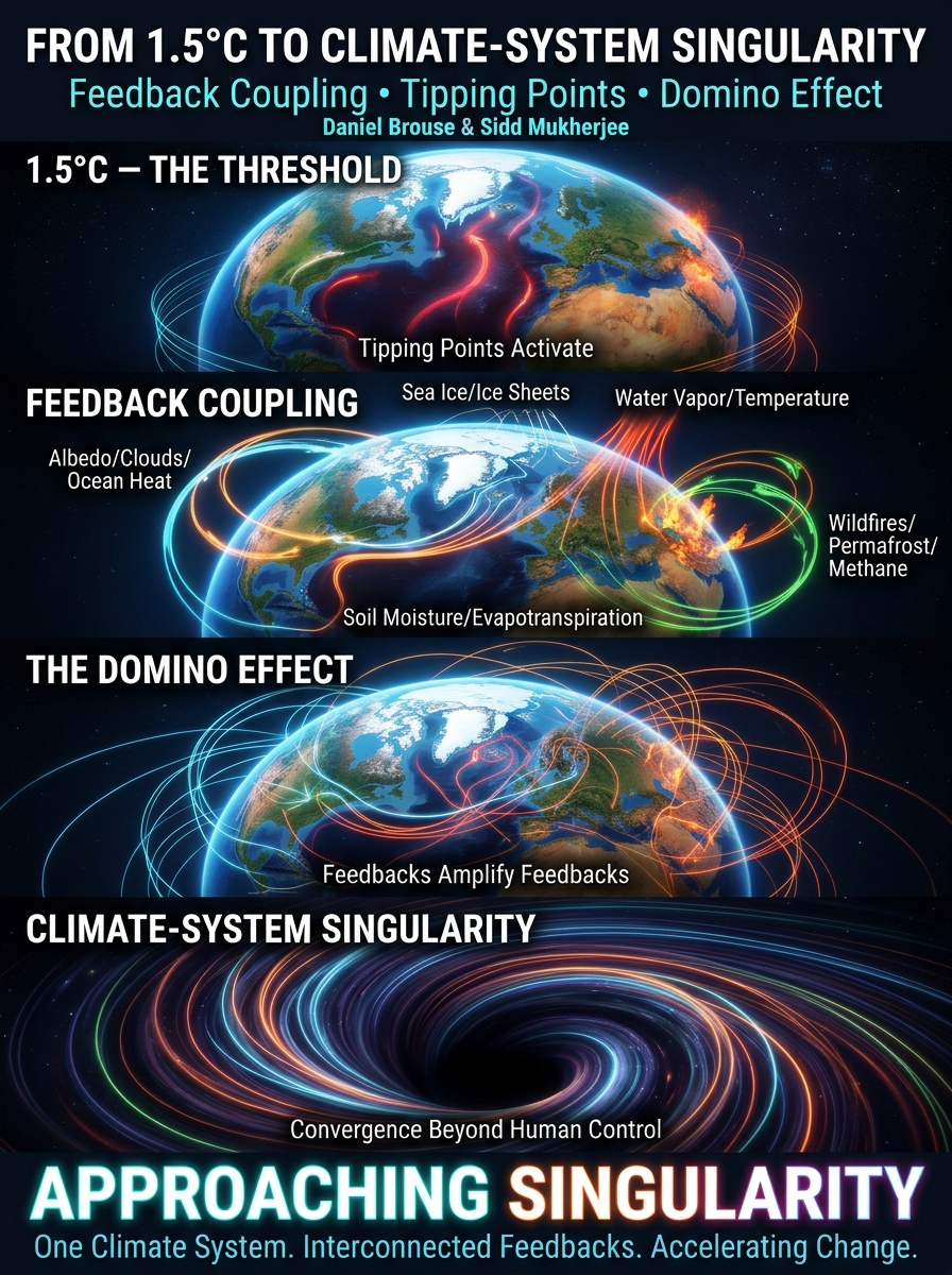
🌎 Approaching Climate-System Singularity

From 1.5°C Warming to Feedback Coupling, Tipping Points, and the Domino Effect

Earth’s climate system is entering a new phase. As global warming exceeds critical thresholds, climate feedbacks increasingly interact, reinforce one another, and trigger cascading changes across the planet.

The Emerging Progression

🌡️ 1.5°C Warming → Increasing pressure on planetary tipping points.

🔄 Feedback Coupling → Climate processes begin reinforcing one another.

🧊 Tipping Points → Ice sheets, oceans, forests, and other systems become increasingly unstable.

🌪️ Domino Effect → Interconnected feedbacks amplify changes across the Earth system.

🕳️ Climate-System Singularity → Feedback networks converge toward increasingly unpredictable and uncontrollable planetary change.

Why It Matters

Climate change is no longer just about rising temperatures. It is about an increasingly interconnected system in which one change amplifies another.

📖 Explore the paper, examine the emerging feedback connections, and discover the scientific sources and research behind this framework.

Feedback Coupling, Tipping Points, and the Domino Effect

1. The 1.5°C Threshold: Tipping Points Activate

The 2023–2026 four-year average is projected to surpass 1.5°C above preindustrial levels. This is no longer simply a projection of future warming. We are observing the consequences of an increasingly interconnected climate feedback system in real time.

Climate Feedback and Tipping-Point Network

2. Feedback Coupling: The Domino Effect

The most observable emerging feedback couplings include:

  • Albedo – low-level clouds – ocean heat content
  • Ocean heat content – sea ice – ice-sheet melting
  • Atmospheric water vapor – temperature – precipitation
  • Soil moisture – evapotranspiration – temperature
  • Wildfire – permafrost – carbon release – methane

As these feedbacks interact, individual climate processes become interconnected, mutually reinforcing drivers of accelerating change.

Observable Climate Feedback Coupling

3. Climate-System Singularity: Convergence of Feedback Networks

As individual feedbacks emerge, couple, and organize into self-reinforcing networks, those networks increasingly interact and converge toward a unified, interconnected climate system.

A climate-system singularity represents a critical tipping point where interacting feedbacks drive increasingly uncontrollable and irreversible planetary change. It is analogous to a gravitational singularity, such as a black hole, where converging forces produce a point beyond which conventional predictions and control break down. In the climate system, this represents a trajectory toward increasingly unpredictable, self-reinforcing change that becomes progressively decoupled from human policy intervention.

Climate-System Singularity


Sources

1. IPCC (2021) — Climate Change 2021: The Physical Science Basis, Chapter 7: Earth’s Energy Budget, Climate Feedbacks, and Climate Sensitivity.
Covers water vapor, clouds, surface albedo, and interconnected climate feedback processes.
IPCC Chapter 7

2. IPCC (2023) — Climate Change 2023: Synthesis Report.
Documents increasing risks of abrupt and irreversible climate changes, including tipping-point risks between 1.5°C and 2.5°C.
IPCC Synthesis Report

3. Global Tipping Points Report (2025).
Comprehensive scientific assessment of interacting Earth-system tipping elements and cascading risks.
2025 Report and downloads

4. Nature Geoscience (2025) — Destabilization of Earth System Tipping Elements.
Examines interactions among Greenland, Antarctic, AMOC, and Amazon tipping elements.
Read scientific paper

5. IPCC (2021) — Chapter 5: Global Carbon and Other Biogeochemical Cycles and Feedbacks.
Covers permafrost, vegetation, soil carbon, ocean carbon exchange, and greenhouse gas feedbacks.
IPCC Chapter 5

6. WMO (2026) — Global Annual to Decadal Climate Update 2026–2035.
Provides current temperature projections and the probability of temporarily exceeding 1.5°C.
WMO Climate Update

Additional research and original work

7. Daniel Brouse and Sidd Mukherjee — Climate Feedback and Tipping-Point Network.
Original research

8. Daniel Brouse and Sidd Mukherjee — Observable Climate Feedback Coupling.
Original research

9. Daniel Brouse — Climate-System Singularity.
Conceptual framework

bookmark_borderTrump, Epstein, Wright: Crimes Against Humanity

Let the investigations kick into high gear—and let clean, renewable energy lead the way! 🌎⚡🌱

At the top of my congressional investigation wish list: Donald Trump, Jeffrey Epstein, Energy Secretary Chris Wright, and potential crimes against humanity connected to climate policy.

The DOE Climate Working Group: Legal Violations, Ideological Networks, and Ecofascist Connections

Overview

Court rulings have established that the Department of Energy’s (DOE) Climate Working Group (CWG) violated the Federal Advisory Committee Act (FACA), a federal law requiring transparency, balanced representation, and public accountability in the operation of federal advisory committees.

The case exposes serious questions about the group’s formation, membership, ideological affiliations, and influence over federal climate policy.

Several individuals associated with the CWG have connections to the CO₂ Coalition, a nonprofit organization that challenges established climate science and promotes arguments emphasizing the benefits of atmospheric carbon dioxide.

The group’s analysis became a foundation for the Trump administration’s effort to overturn the EPA Endangerment Finding, a cornerstone of federal climate regulation. That reversal provided the administration with a basis for dismantling major climate and pollution protections.

The connections among the DOE, the CWG, fossil fuel interests, and individuals appearing in the Epstein files demand congressional investigation. Those connections include reported associations involving members of the administration and the broader climate-policy network.

Chris Wright: Fossil Fuel Industry to Secretary of Energy

Chris Wright (born January 15, 1965) is an American businessman and politician serving as the 17th U.S. Secretary of Energy.

His professional background is rooted in the fossil fuel industry.

Business Background

Liberty Energy

Wright founded and formerly served as CEO of Liberty Energy, a Denver-based energy company that became North America’s second-largest hydraulic fracturing (fracking) company.

Pinnacle Technologies

Founded in 1992, Pinnacle Technologies helped pioneer the hydraulic fracture mapping industry.

Wright’s transition from fossil fuel industry leadership to directing federal energy policy places his professional interests and policy decisions squarely within the scope of congressional oversight.

The Investigative Report: From Climate Denialism to Ecofascist Ideology

I began investigating climate denialism and the CO₂ Coalition in the spring of 2025, tracing its connections to the Department of Energy’s Climate Working Group.

My initial hypothesis centered on financial interests: fossil fuel companies and affiliated organizations fund campaigns that challenge established climate science, protect existing investments, and delay environmental regulation.

That financial motive explains part of the pattern. It does not explain the entire network.

The release of the Epstein files introduced another dimension to the investigation. Correspondence, affiliations, and publicly documented rhetoric raised questions about the intersection of elite networks, population ideology, eugenics, and environmental collapse.

The investigation therefore expanded beyond conventional climate denialism to examine the relationship between fossil fuel interests and ecofascist ideology.

Ecofascism: Environmental Collapse as a Tool of Human Elimination

Ecofascism combines environmental ideology with authoritarian hierarchy, racialized survival theories, eugenics, and the belief that certain populations are expendable.

Rather than treating environmental destruction as a threat to humanity, this ideology rationalizes unequal human survival and frames population reduction through catastrophe as beneficial.

The distinction is fundamental:

  • Climate denialism: Protects economic and political interests by undermining climate science and delaying environmental protections.
  • Eugenics: Assigns unequal value to human lives based on inherited characteristics and perceived human worth.
  • Ecofascism: Combines environmental collapse with authoritarian and eliminationist population ideology.

These ideas warrant examination wherever they intersect with political influence, environmental policy, and elite networks.

Epstein’s Publicly Released Statements

Publicly released statements attributed to Jeffrey Epstein include:

“I liked the argument that more CO₂ is good for plants.”

This statement echoes a central argument promoted by the CO₂ Coalition: that increased atmospheric carbon dioxide benefits vegetation through its role in plant growth.

However, the physiological benefits of additional CO₂ do not negate the destructive consequences of accelerating climate change, including extreme heat, drought, ecosystem disruption, and damage to agricultural systems.

Other statements attributed to Epstein reveal an explicit interest in population reduction, eugenics, and racial hierarchy:

“Maybe climate change is a good way of dealing with overpopulation—the earth’s forest fire. Potentially a good thing for the species.”

“Executions of the elderly and infirm make sense.”

“African music has lots of beats and little development—not an accident. It mirrors their learning process.”

These statements, if accurately attributed and understood in their documentary context, expose a worldview that extends far beyond conventional environmental policy disagreement.

They invoke population elimination, the devaluation of vulnerable people, and racialized judgments about human capability.

The Central Investigative Question

This investigation concerns more than climate science or fossil fuel industry influence.

It concerns the intersection of money, political power, ideological networks, environmental policy, and the unequal valuation of human life.

Financial interests can explain efforts to undermine climate science and obstruct regulation. Eugenic and eliminationist rhetoric raises a separate and deeply troubling question: whether environmental catastrophe is being rationalized within ideological networks that assign different values to different human populations.

The DOE Climate Working Group’s documented legal violations, its connections to climate-denial organizations, the administration’s reliance on its work, and the wider network of reported associations warrant a comprehensive congressional investigation.

Climate policy must serve humanity—not fossil fuel profits, authoritarian ideology, or theories that treat human lives as expendable.

The investigations need to follow the evidence, trace the money, expose the networks, establish accountability, and protect the public interest.

And the solution is clear: let clean, renewable energy lead the way.

SOURCES

bookmark_borderEl Niño and the U.S. Economy: Inflation Risks Rise in 2027

by Daniel Brouse

EL NIÑO: THE ECONOMIC RIPPLE EFFECTS

A 1-Percentage-Point Inflation Increase Could Cost Households, Increase Federal Spending, and Add Trillions to the National Debt

Federal Reserve research examines how El Niño can affect inflation, employment, household purchasing power, and the broader U.S. economy.

A new study from the Federal Reserve Bank of San Francisco identifies a significant economic risk associated with the current El Niño episode: U.S. inflation could increase by as much as 1 percentage point in 2027.

Although the initial price effects of the current episode are projected to fade by the end of 2026, historical estimates suggest that longer-term inflationary effects could emerge during 2027. These effects are linked primarily to core services and food prices, with the magnitude influenced partly by whether a La Niña episode follows El Niño.

The study also identifies potential employment gains, which may be widespread across industries and states during the year following El Niño.

An additional percentage point of inflation may sound relatively small, but its economic consequences extend far beyond higher grocery bills. It affects household purchasing power, government expenditures, interest rates, federal deficits, and the national debt.

1. What a 1-Percentage-Point Increase in Inflation Means for Household Budgets

The Federal Reserve study identifies an inflationary effect of as much as 1 percentage point in 2027.

Based on U.S. Bureau of Labor Statistics consumer expenditure data, the average American consumer unit spent approximately $78,535 annually in 2024.

An additional 1 percentage point of inflation, relative to the baseline, would translate into approximately $785 in additional annual household expenses, or about $65 per month.

Additional household expenseAmount
Monthly$65.45
Annual$785
Five years$3,927
Ten years$7,854

Illustrative calculations assume the additional 1% price-level difference persists, without further compounding.

The actual impact will vary depending on household spending patterns, particularly exposure to food, housing, transportation, and services.

The important distinction is that even when inflation subsequently slows, the higher price level generally remains. A reduction in the inflation rate does not reverse the previous price increases.

2. The National Economic Impact

The BLS reports approximately 135.76 million U.S. consumer units.

Applying the additional 1% expenditure to the national average produces an estimated:

$106.6 billion in additional annual household spending.

This is an illustrative national extrapolation, not a forecast of actual consumer spending. It demonstrates the potential economic scale of a relatively small change in the overall price level.

The consequences extend beyond consumer purchases:

  • Prices rise faster than otherwise expected.
  • Households pay more for food, services, and other necessities.
  • Higher price levels generally persist even after inflation subsequently slows.
  • Families whose incomes fail to keep pace with inflation experience declining purchasing power.

The effects also extend into employment, business operating costs, government expenditures, and financial markets.

3. Inflation and the Federal Budget

The combination of higher inflation and higher interest rates creates another economic challenge: the cost of financing the federal government.

The government faces pressure from two directions simultaneously.

Higher inflation increases government expenditures.

Social Security cost-of-living adjustments, federal contracts, military procurement, healthcare expenditures, and other government programs can become more expensive.

Higher interest rates increase the cost of financing the national debt.

As Treasury securities mature, the government must refinance portions of its outstanding debt at prevailing market rates. New borrowing also becomes more expensive.

The consequences extend beyond the immediate federal budget because additional interest payments contribute to future deficits and borrowing requirements.

The United States already carries an enormous national debt. Even relatively small changes in borrowing costs can translate into substantial additional federal expenditures.

4. What the Congressional Budget Office Estimates

The Congressional Budget Office (CBO) has examined how changes in inflation and interest rates affect federal revenues, expenditures, and deficits.

Its April 2026 analysis, How Changes in Economic Conditions Might Affect the Federal Budget: 2026 to 2036, provides useful estimates.

CBO examined a scenario in which inflation and nominal interest rates were each 0.1 percentage point higher every year than projected in its baseline forecast.

The resulting estimates include:

Federal budget impactAdditional cost
Cumulative deficits, 2027–2036$311 billion
Higher direct interest costs$339 billion
Additional interest from increased borrowing$48 billion

The $311 billion figure represents the estimated net increase in cumulative deficits, not the sum of the interest-cost components.

CBO’s sensitivity methodology provides a way to examine the potential consequences of larger changes.

For perspective, scaling its combined inflation-and-interest-rate scenario to a sustained 1-percentage-point increase in both variables produces an illustrative estimate of approximately:

$3.11 trillion in additional federal deficits over ten years.

This is a sensitivity calculation based on CBO’s model, not a prediction of the fiscal consequences of the current El Niño episode. It assumes the changes persist relative to the baseline throughout the projection period.

CBO also separately estimates that a sustained 0.1-percentage-point increase in interest rates alone would add approximately $379 billion to cumulative deficits over the same decade.

These scenarios should not be added together because they represent different economic assumptions.

5. The National Debt Feedback Loop

Inflation and interest rates can reinforce existing fiscal pressures.

The inflation-debt spiral:

  1. Higher inflation increases government expenditures.
  2. Higher interest rates make Treasury refinancing more expensive.
  3. Larger expenditures and interest payments increase federal deficits.
  4. Larger deficits require additional government borrowing.
  5. Additional borrowing increases the national debt.
  6. More debt eventually requires additional interest payments.

The result is increasing interest obligations and greater fiscal pressure.

This does not mean every increase in inflation automatically produces an equivalent increase in interest rates. Monetary policy, economic growth, Treasury market conditions, and inflation expectations all influence the outcome.

However, the combination presents a significant risk to long-term fiscal stability.

6. What Does This Mean for Taxpayers?

The consequences extend well beyond the federal budget.

  • More tax revenue is directed toward servicing debt rather than public services and investment.
  • Future taxpayers inherit higher debt-service obligations.
  • Government borrowing competes with private investment for available capital.
  • Higher borrowing costs can affect mortgages, business loans, and consumer credit.
  • The government’s ability to respond to future economic emergencies becomes more constrained.

A 1-percentage-point increase in inflation accompanied by a 1-percentage-point increase in interest rates has implications for federal spending, debt financing, and future taxation.

The approximately $3.11 trillion CBO sensitivity calculation illustrates the potential scale of the problem under sustained changes in both variables. It should not be interpreted as the actual projected cost of El Niño.

The outcome depends on how long inflation persists, how Treasury yields respond, and how quickly outstanding federal debt reprices.

7. Climate and Economics: The Bigger Picture

The economic implications of El Niño demonstrate how climate patterns can influence more than agriculture and weather-related disruptions.

They can affect:

  • Consumer prices and household purchasing power.
  • Employment and labor markets.
  • Government expenditures and federal deficits.
  • Interest rates and the cost of financing debt.
  • Long-term economic stability.

The economic implications of climate change extend well beyond the direct costs of storms, droughts, flooding, and extreme temperatures.

El Niño provides another example of how climate variability can transmit economic pressure through interconnected systems.

Climate risk is economic risk.

Understanding these connections is increasingly important for forecasting inflation, evaluating fiscal exposure, managing financial risks, and planning for the years ahead.


Original Research and Sources

Federal Reserve Bank of San Francisco

In Hot Water? The Macroeconomic Impacts of El Niño

Brigitte Roth Tran, Working Paper 2026-21, October 13, 2026.

U.S. Bureau of Labor Statistics

Consumer Expenditures in 2024

Source for average annual household expenditures and the number of consumer units.

Congressional Budget Office

How Changes in Economic Conditions Might Affect the Federal Budget: 2026 to 2036

Source for federal budget sensitivity to inflation and interest-rate changes.

bookmark_borderThe $6.3 Billion Binance Heist: North Korean Accusations and Questions About Trump’s Pardon

The world’s largest cryptocurrency exchange, Binance, was struck by a massive $6.3 billion cyber heist on Thursday, October 29, 2026. The theft ranks as the largest cryptocurrency heist in history.

Multiple leading cryptocurrency analytics firms and security agencies have formally accused North Korea of orchestrating the $6.3 billion theft. These allegations raise serious questions about the scale of the operation, the perpetrators, and the potential geopolitical implications of an attack of this magnitude.

On October 23, 2025, President Donald Trump pardoned Binance founder and former CEO Changpeng “CZ” Zhao, who had previously pleaded guilty to violating the Bank Secrecy Act. Zhao’s prosecution involved Binance’s failure to maintain an effective anti-money-laundering program.

White House Press Secretary Karoline Leavitt defended the pardon, stating that the Biden administration had prosecuted Zhao as part of its purported “war on cryptocurrency.”

The timing and circumstances of Trump’s pardon now raise even more serious questions in the wake of the Binance heist and the reported involvement of a North Korean state-sponsored hacking operation.

Is Trump complicit in aiding and abetting North Korea, directly or indirectly, by granting clemency to Binance’s founder? What responsibility, if any, does the administration bear for the consequences of that decision?

And given the alleged involvement of a hostile foreign government in a theft of this unprecedented magnitude, should the attack be examined not only as a massive international financial crime, but also under the legal frameworks governing acts of war, cyberwarfare, and crimes against humanity?

The allegations against North Korea are substantial. TRM Labs says it has high confidence in its attribution to the North Korean hacking unit TraderTraitor, and Chainalysis and other investigators have also pointed to North Korea.

Relevant reporting and documentation:

bookmark_borderFlood-Risk Disclosure Is Financial Risk Management: Pennsylvania’s New Law and the Growing Climate Liability of Real Estate

By Daniel Brouse and Sidd Mukherjee

Insurance and Real Estate | Financial Analysis | Independent Climate Research | Physics and Climate Systems

Overview

🏠 PENNSYLVANIA’S NEW FLOOD-RISK DISCLOSURE LAW: WHAT HOME BUYERS NEED TO KNOW

A home may be your biggest investment. Do you know its flood risk—and whether your insurance will cover the damage?

Pennsylvania’s new flood-risk disclosure law brings an important issue into focus: flood risk is not just an environmental problem. It is an insurance, real estate, financial planning, and consumer protection issue.

The paper, Flood-Risk Disclosure Is Financial Risk Management: Pennsylvania’s New Law and the Growing Climate Liability of Real Estate, Daniel Brouse and Sidd Mukherjee, examine the implications of this legislation and why informed property decisions matter.

Drawing on previous work in insurance, real estate, financial analysis, physics, and climate research, the paper explores:

• What Pennsylvania’s new law means for home buyers and sellers.

• Why standard homeowners insurance generally does not cover flood damage.

• How flood exposure can affect property values, insurance costs, and household finances.

• Why historical flood records alone cannot fully establish future risk.

• How climate change, better disclosure, insurance planning, and practical mitigation fit together.

• Why renters, existing homeowners, and taxpayers also have a stake in flood-risk awareness.

The bottom line: A property’s purchase price tells only part of the story. Buyers need to understand the risks, insurance limitations, and potential future expenses associated with owning it.

The conclusion is simple: Know the risks. Protect your investment. Build more resilient communities.

#FloodRisk #Pennsylvania #RealEstate #Insurance #ClimateChange #ConsumerProtection #ClimateAdaptation

Introduction

Pennsylvania’s new flood-risk disclosure law recognizes a fundamental principle of responsible financial decision-making: people cannot adequately evaluate a property’s financial risks when material information about those risks is unavailable or undisclosed. Signed into law on October 22, 2026, House Bill 1704 strengthens residential real estate disclosures concerning flood history, flood insurance, and related risk factors. The law also directs the Pennsylvania Insurance Department to provide public information about flood risks, mitigation, and insurance options.

This legislation has implications extending well beyond real estate transactions. Flood risk affects property valuation, mortgage lending, insurance adequacy, household financial security, municipal budgets, and taxpayer exposure. Climate change adds another dimension by altering the conditions under which property risks must be evaluated. Historical flood records and existing hazard maps are important, but they cannot, by themselves, establish the full range of future risks.

Drawing on decades of experience in insurance, real estate, financial analysis, and independent climate research, this paper argues that Pennsylvania’s legislation is an important step toward more informed property transactions. It also identifies the limitations of disclosure alone and the need for integrated climate-risk assessment, transparent insurance information, forward-looking property valuation, and financially responsible adaptation.

1. Introduction: The Financial Consequences of Undisclosed Risk

Pennsylvania has taken an important step toward protecting homebuyers from financial losses they may not anticipate when purchasing residential property.

On October 22, 2026, Governor Josh Shapiro signed House Bill 1704 into law. As reported by WHYY on October 27, the legislation expands the information residential property sellers must disclose about flooding and related risks. Compliance with the revised disclosure requirements is scheduled for the summer of 2028. WHYY’s report on the new law.

The underlying issue is straightforward: purchasing a home is one of the largest financial commitments most households make. Buyers need accurate information about the property’s condition, operating expenses, insurability, and exposure to foreseeable losses. When important risks are not adequately communicated, buyers can make decisions based on an incomplete assessment of the property’s true financial cost.

My professional experience spans real estate, mortgage banking, financial planning, accounting, and financial analysis. My independent climate research, which began in 1992, has focused on the physical processes driving climate change and the implications of a changing climate for human systems.

These fields converge on a common principle: risk that is omitted from a financial decision does not disappear. It remains a potential liability.

Flood-risk disclosure is therefore not simply a paperwork requirement. It is part of the larger responsibility to ensure that property buyers, lenders, insurers, and communities can make informed decisions about the assets and liabilities they assume.

2. What Pennsylvania’s New Law Requires

House Bill 1704 amends Pennsylvania’s residential real estate disclosure provisions under Title 68 of the Pennsylvania Consolidated Statutes.

The legislation strengthens the information buyers receive about flood-related risks. Among the provisions described in the enacted legislation and WHYY’s reporting are requirements concerning:

  • The number of times a property has experienced flooding and the estimated dates of those incidents.
  • Whether a property is located in a Federal Emergency Management Agency-designated high- or moderate-risk flood zone.
  • Whether flood insurance is required for the property.
  • Whether the seller has received government assistance for flood damage.
  • Whether the seller has filed a flood insurance claim.

The law also directs the Pennsylvania Insurance Department to publish information about flood-risk factors, mitigation measures, insurance coverage, and resources for identifying properties in flood-hazard areas.

The revised disclosure process will include a written notice advising prospective buyers that many Pennsylvania properties face flood risks and that standard homeowners insurance typically does not cover flood damage. Buyers are encouraged to consult insurance professionals and investigate separate flood coverage.

These requirements are significant because they connect property disclosures with practical financial decisions. Buyers need to know not only whether a property has flooded but also whether the insurance they expect to protect their investment will actually cover the loss.

The important distinction is between knowing that a risk exists and understanding the financial consequences of that risk. Effective disclosure should help buyers investigate both.

Sources: Pennsylvania House Bill 1704 and the Pennsylvania Insurance Department’s announcement.

3. The Insurance Problem: Homeowners Coverage Is Not Flood Coverage

One of the most consequential misconceptions in residential property ownership is that a standard homeowners insurance policy covers every major source of property damage.

It does not.

Standard homeowners policies generally exclude flood damage. Flood insurance is typically purchased separately, either through the National Flood Insurance Program or an eligible private insurer. Coverage terms, exclusions, limits, deductibles, and eligibility vary by policy.

This distinction can have severe financial consequences.

A buyer may purchase a home, obtain a mortgage, and maintain homeowners insurance while remaining exposed to substantial flood losses. The existence of an insurance policy does not establish that the property is adequately insured against every material hazard.

From an insurance and financial-planning perspective, this is a problem of incomplete risk transfer. The homeowner retains a potentially substantial uninsured liability.

A flood can damage structural components, electrical systems, heating and cooling equipment, appliances, flooring, furnishings, and personal possessions. Recovery may involve temporary housing, repairs, reconstruction, and expenses that continue while a property is uninhabitable. Actual coverage depends on the applicable policies and circumstances.

The financial consequences extend beyond the initial repair bill. Flood damage may affect resale value, future insurance costs, mortgage affordability, and the amount of money a household can preserve for retirement or other needs.

This is why the insurance question must be addressed before a transaction closes.

Buyers should determine:

  1. What hazards the homeowners policy covers and excludes.
  2. Whether separate flood insurance is available and appropriate.
  3. What the policy limits, deductibles, exclusions, and waiting periods are.
  4. Whether the coverage is sufficient to address the property’s actual replacement and recovery costs.
  5. How premiums and other carrying costs affect the household’s long-term budget.

Pennsylvania’s new law directs attention to these questions. Its broader value will depend on whether buyers use the information to evaluate their actual exposure rather than treating disclosure as another form to sign.

4. Real Estate Valuation Must Account for Risk

Real estate valuation is not simply a matter of comparing square footage, location, amenities, and recent sales.

A property’s economic value also depends on the costs and risks associated with owning it.

Flood exposure can affect insurance premiums, repair and maintenance expenses, financing conditions, marketability, and the potential for future losses. Two otherwise comparable properties may therefore have materially different economic profiles.

A waterfront home, for example, may offer exceptional recreational value, scenic views, and personal enjoyment. Those benefits may justify a higher purchase price for a particular buyer. However, the same property may carry additional insurance expenses, mitigation costs, and exposure to flooding.

There is no universal answer to whether a property with elevated flood risk is a good investment. That determination depends on the buyer’s objectives, financial resources, risk tolerance, insurance options, and the property’s specific characteristics.

The essential requirement is informed consent to the financial risk.

My experience in real estate and mortgage banking reinforces the importance of distinguishing a property’s purchase price from its total cost of ownership. A transaction can appear affordable at closing while creating substantial future expenses that were not incorporated into the buyer’s original budget.

A more complete financial assessment should consider:

  • Purchase price and financing costs.
  • Property taxes and ordinary maintenance.
  • Homeowners and flood insurance premiums.
  • Expected mitigation and resilience investments.
  • Potential deductibles and uninsured losses.
  • The implications of future hazard changes for resale and financing.

Not every risk can be expressed as a precise dollar amount. Nevertheless, acknowledging uncertainty is better financial practice than treating an incomplete estimate as a comprehensive valuation.

A property’s market price does not automatically reflect its full climate-related financial risk.

Improved disclosures can help correct that information gap, although disclosure alone cannot guarantee that prices, insurance premiums, or lending decisions will fully reflect future exposure.

5. Climate Change Changes the Risk-Assessment Problem

Flood risk is not determined by property history alone. It also depends on precipitation, drainage, topography, river conditions, coastal processes, land development, infrastructure, and the changing physical environment.

Climate change adds an important consideration: historical conditions are not necessarily a complete guide to future conditions.

Warmer air can hold more water vapor, increasing the potential for heavier precipitation under suitable atmospheric conditions. Changes in precipitation patterns can affect runoff, streamflow, drainage systems, and flood hazards. The resulting effects vary by location and depend on local geography, infrastructure, and other factors.

At the same time, flooding can occur outside formally designated high-risk zones. Localized rainfall, overwhelmed drainage systems, changing waterways, and other conditions can produce losses that a buyer might not anticipate from a single map or a property’s previous history.

This does not mean every property will experience increasing flood risk at the same rate. Nor does climate change eliminate the value of historical flood records or FEMA flood maps. Both remain important sources of information.

It means that risk assessment should consider multiple sources of evidence and distinguish present conditions from future possibilities.

My climate research has focused on the interaction of climate processes, feedbacks, and changes in the Earth’s energy system. That work informs a broader concern about financial risk: physical systems can change, and risk assessments that assume past conditions will continue indefinitely can become inadequate.

The appropriate response is not to disregard established flood maps. It is to use them alongside other relevant information, including local flood histories, drainage conditions, infrastructure assessments, updated hazard analyses, and credible forward-looking projections.

For real estate, the distinction is critical. A disclosure based on what a seller knows about past flooding serves a different purpose from a scientific assessment of what could happen to the property over the coming decades.

Historical disclosure documents the past. Climate-informed risk assessment helps evaluate the future. Both are necessary for sound decisions.

6. Disclosure Is Consumer Protection and Fiscal Responsibility

The economic benefits of better disclosure extend beyond individual buyers.

When a homeowner experiences a major uninsured loss, the consequences may include depleted savings, additional borrowing, delayed repairs, mortgage distress, or the loss of accumulated household wealth.

Public assistance may help some affected households, but disaster assistance is not a substitute for comprehensive insurance and does not guarantee full compensation for losses.

Flood damage can also affect local governments through emergency response expenses, infrastructure repairs, drainage improvements, and other recovery costs. Public insurance programs and disaster assistance may expose taxpayers to additional financial obligations.

These consequences connect private property decisions to public fiscal responsibility.

Better disclosure can help buyers make more informed choices about whether to purchase a property, obtain insurance, invest in mitigation, or reconsider the transaction. It can also encourage earlier investments in measures that reduce potential losses.

Depending on the property and hazard, mitigation may include improving drainage, protecting critical equipment, installing appropriate flood-resistant materials, elevating vulnerable components, or undertaking professionally designed structural improvements.

Not every mitigation measure is appropriate for every property, and its cost-effectiveness should be evaluated individually.

Nevertheless, identifying a risk before a loss occurs generally provides more opportunities to plan than discovering it after the damage is done.

Pennsylvania’s legislation addresses one part of this problem by strengthening the flow of information between sellers and buyers. The next challenge is to ensure that the information supports practical decisions rather than merely satisfying a disclosure requirement.

7. The Remaining Gap: Renters and Existing Property Owners

The new law primarily addresses residential property sales. It does not establish a comparable general flood-risk disclosure requirement for landlords and renters.

That distinction matters.

Renters can face serious financial consequences from flooding, including damage to personal belongings, displacement, temporary housing expenses, and interruptions to employment or daily life. A landlord’s building insurance does not necessarily cover a tenant’s personal possessions or additional living expenses.

Tenants may also have limited control over building-level mitigation measures and may not know whether a property has flooded previously.

The absence of equivalent disclosure requirements for renters leaves an important consumer-information gap. WHYY reports that a separate proposal concerning flood disclosures for rental properties had not advanced beyond committee referral as of its October 27, 2026, report.

A comprehensive approach to flood-risk communication should consider both owners and tenants, while distinguishing the respective responsibilities of property owners, insurers, and occupants.

Existing homeowners also need access to understandable information about their current exposure. They should not have to wait until they sell their homes to discover that their insurance coverage is inadequate or that local flood conditions warrant further investigation.

The public information resources required by House Bill 1704 can help address this broader need, provided they remain accessible, useful, and responsive to changing information.

8. Recommendations for a More Comprehensive Approach

Pennsylvania’s new law creates an opportunity to strengthen the relationship between real estate transactions, insurance decisions, climate adaptation, and financial planning.

Several additional measures would build on its foundation.

A. Make flood-risk information accessible before an offer is made

Buyers should be encouraged to investigate flood history, mapped hazards, insurance requirements, and available coverage early in the purchasing process. Discovering significant costs after making a binding commitment can leave buyers with fewer practical options.

B. Distinguish historical records from forward-looking risk

Disclosure forms should communicate what is known about past flooding without implying that a property with no documented history is free from risk. Public resources should help buyers understand the limitations of historical records and hazard maps.

C. Encourage insurance review before closing

Buyers should obtain quotes and review relevant policy terms before finalizing a purchase. This allows insurance costs, deductibles, exclusions, and coverage availability to inform the household budget and purchase decision.

D. Incorporate climate risk into property and infrastructure planning

Local governments, lenders, insurers, and property owners should evaluate relevant forward-looking hazard information when making long-term decisions. The appropriate analysis will differ between inland river flooding, localized stormwater flooding, and coastal exposure.

E. Expand consumer education

Disclosure is most effective when people understand what the information means. Public education should explain the difference between homeowners insurance and flood insurance, how to investigate risk, what mitigation can accomplish, and where to obtain qualified advice.

F. Evaluate affordability and financial feasibility

Some households have limited alternatives when searching for affordable housing. Better information cannot, by itself, resolve that constraint. Policy responses should recognize the need to balance risk awareness with practical access to housing and the cost of mitigation and insurance.

G. Improve transparency across the property lifecycle

Risk information should not be viewed solely as a requirement at the point of sale. Property owners, renters, insurers, lenders, and local officials all benefit from accessible information that supports ongoing risk management.

These recommendations are consistent with a basic principle of financial analysis: identify material risks, estimate their potential consequences, evaluate the available responses, and make decisions with a clear understanding of the remaining uncertainty.

9. Integrated Climate Stewardship and Property Risk

My broader approach to climate solutions is called Integrated Climate Stewardship. It emphasizes reducing avoidable resource consumption and climate impacts while directing resources toward practical benefits and resilience.

Applied to real estate, this framework supports a comprehensive approach to property risk rather than treating flood disclosure, insurance, energy use, infrastructure, and climate adaptation as unrelated issues.

A property is part of a larger system. Its financial performance depends not only on the building itself but also on the surrounding environment, public infrastructure, insurance market, utilities, and community resilience.

The same principle applies to climate risk. Effective management requires attention to both the physical hazard and the economic systems that determine who bears the losses.

For an individual homeowner, that may mean evaluating insurance coverage, reducing avoidable exposure, and making cost-effective improvements. For a community, it may mean improving drainage, maintaining infrastructure, updating hazard assessments, and evaluating development decisions against long-term risks.

For lenders and insurers, it means recognizing that reliable risk information is essential to assessing potential losses. For policymakers, it means considering the distribution of costs among property owners, private insurers, public programs, and taxpayers.

This is not an argument that every climate-related risk can be eliminated. It is an argument that avoidable financial exposure should not be ignored simply because the relevant costs may occur years after a transaction.

10. Conclusion: Disclosure Is the Beginning, Not the End

Pennsylvania’s new flood-risk disclosure law establishes an important principle for residential real estate: prospective buyers deserve more complete information about a property’s flood history and related insurance considerations.

That principle aligns with longstanding practices in responsible insurance, real estate, and financial analysis. A major financial commitment should be based on an informed assessment of material risks, not merely on the purchase price or the assumption that existing insurance covers every foreseeable loss.

The legislation is a meaningful step, but its limits must be understood. Disclosure does not prevent flooding, guarantee affordable insurance, eliminate uninsured losses, or ensure that property values accurately reflect future climate conditions. Its effectiveness will depend on implementation, public understanding, and the decisions that buyers and other stakeholders make with the information provided.

Climate change adds urgency to the broader question of how society evaluates long-lived assets. Homes, mortgages, infrastructure, and insurance arrangements often extend across decades. Risk assessments that rely exclusively on past conditions can leave households and institutions exposed when relevant conditions change.

My experience in insurance, real estate, mortgage banking, financial analysis, and climate research leads to one central conclusion:

Sound property ownership requires more than knowing what a home costs today. It requires understanding the risks, liabilities, and future expenses that come with owning it.

Pennsylvania’s new law moves the state toward that objective. The next step is to connect better disclosure with informed insurance decisions, climate-aware valuation, practical mitigation, and financially responsible planning.

The goal should be straightforward: fewer preventable losses, better-informed buyers, more resilient communities, and less avoidable financial risk for homeowners and taxpayers alike.


Sources and Further Reading

  1. Sophia Schmidt, “Gov. Shapiro signs law requiring home sellers to disclose more about a home’s flood risk,” WHYY, October 27, 2026.
  2. Pennsylvania General Assembly, House Bill 1704, 2025–2026 Regular Session.
  3. Pennsylvania Insurance Department, “Governor Shapiro Signs New Law to Improve Transparency for Homeowners and Protect Pennsylvanians from Unexpected Flood Losses,” October 23, 2026.
  4. Commonwealth of Pennsylvania, Do I Need Flood Insurance?.

This paper presents professional and analytical commentary on flood-risk disclosure, insurance, real estate, and climate adaptation. It is not legal, insurance, investment, or property-specific advice.

bookmark_borderAI, Productivity, Sustainability, and You

Why the Age of Artificial Intelligence Requires a New Economic Model

By Daniel Brouse

The Economic Challenge of Artificial Intelligence

We need a new economic model that separates people’s ability to earn a living from the necessity of working for a living.

As artificial intelligence (AI) and automation transform the economy, traditional employment may no longer provide a reliable source of income for everyone. Machines can increasingly perform tasks that once required human labor, raising productivity while potentially eliminating jobs and weakening the link between employment and economic security.

One approach worth serious consideration is a $60,000 annual government stipend per person, funded in part by taxing pollution while eliminating income taxes. This would shift the tax burden away from human productivity and toward activities that impose environmental costs, while providing people with a more secure share of the economy’s productive output.

This is a proposed economic model, not an established policy. Its implementation would require careful consideration of funding, inflation, eligibility, existing public benefits, and the distribution of economic gains.

The Productivity and Disinflation Wildcard

Another important variable is the relationship between productivity gains and disinflation.

AI-driven improvements in productivity and efficiency could sharply reduce the cost of producing goods and services. As automation reduces labor requirements and technological advances improve resource utilization, prices could decline even as total economic output increases.

This creates an important possibility: We could produce more while requiring less human labor and fewer resources.

If these productivity gains translate into lower consumer prices, a given income could purchase more goods and services. The result could be a substantial improvement in living standards, provided the benefits reach consumers rather than being captured primarily as corporate profits.

However, lower production costs do not automatically translate into lower prices. Market competition, ownership, energy costs, access to resources, and corporate pricing decisions will influence how much of the savings consumers receive. Nor does greater productivity guarantee that every sector will experience falling prices.

The central economic challenge is to ensure that the benefits of technological progress are broadly shared rather than concentrated among a small number of business owners and investors.

We cannot stop technological progress, but we can redesign our economic system to distribute its benefits more equitably.

Global Responses: Policies Already Under Consideration

The economic transition driven by AI is not a distant possibility. It is already underway. Governments worldwide are considering different ways to address technological disruption, economic inequality, and the distribution of productivity gains.

These initiatives differ in their objectives and scope. Some involve direct cash payments, others explore basic income, and still others seek to capture more public revenue from digital economic activity. They provide examples of the policy options emerging as governments respond to a changing economy.

Taiwan: Proposed Cash Distribution

In August 2026, President Lai Ching-te announced plans for a NT$10,000 cash payment to eligible residents through the 2027 budget. The government cited strong economic growth driven by global demand for AI-related products and sought to share some of the benefits of that growth.

The proposal was referred for legislative review in October 2026. The planned distribution should therefore be understood as a proposed measure, not a completed payment program.

European Union: Debate Over AI Taxation

European policymakers and tax experts are examining how AI-driven automation could erode payroll-tax revenue used to fund pensions, healthcare, and other social programs.

Proposals include shifting more taxation toward corporate profits and exploring ways to capture economic value generated by AI. Direct taxation of AI systems or AI-generated work has also entered the policy debate, although no EU-wide AI-worker tax has been enacted.

The underlying concern is straightforward: If machines perform a growing share of economically valuable work, governments may need to reconsider how they fund public services traditionally financed through taxes on human employment.

South Korea: Basic-Income Proposals

South Korean political leaders, including Lee Jae-myung, have advocated basic-income policies amid concerns about economic inequality, automation, and employment disruption.

These proposals reflect a broader debate about whether traditional employment-based income distribution will remain adequate as AI changes the relationship between labor, productivity, and economic output.

The policy question is how to ensure that technological progress improves living standards across society, including for people whose jobs are displaced or whose bargaining power declines.

The Marshall Islands: Nationwide Universal Basic Income

In November 2025, the Marshall Islands launched its ENRA universal basic income program, providing regular distributions to eligible citizens.

The program uses multiple payment channels, including a dedicated digital wallet. It demonstrates how modern financial infrastructure can support nationwide cash transfers.

The program is funded through the country’s Compact Trust Fund rather than an AI-specific tax. Although it was not created as a response to AI-driven unemployment, it provides a real-world example of a government implementing regular, broadly distributed public payments.

Kenya: Taxation of the Digital Economy

Kenya has pursued taxation of digital economic activity as governments seek to capture revenue from an increasingly digital global economy.

In December 2024, Kenya replaced its 1.5% digital services tax with a 3% significant economic presence tax applying to qualifying nonresident digital businesses, subject to the relevant rules.

This approach illustrates one way to tax economic activity that may not fit traditional models of physical presence and employment. It is not specifically an AI tax or a universal basic-income funding mechanism, but it contributes to the broader discussion about how tax systems must evolve as technology changes how businesses generate revenue.

The United States: A Proposed AI Sovereign Wealth Fund

In June 2026, Senator Bernie Sanders introduced the American AI Sovereign Wealth Fund Act, proposing public ownership of a portion of qualifying AI companies through a federally managed sovereign wealth fund.

The proposal calls for a one-time transfer of 50% of the stock of qualifying AI companies with at least $200 million in annual AI sales. The fund would hold these shares and distribute public benefits, including annual dividends, while supporting priorities such as healthcare, education, and housing.

The legislation remains a proposal, not enacted law. Its approach differs from a universal stipend funded through environmental taxation, but it addresses the same fundamental question: Who should benefit from the wealth created by increasingly powerful technologies?

A sovereign wealth fund could give the public a direct financial stake in AI-generated economic value. A universal stipend funded through taxation would pursue a similar distributional objective through a different mechanism.

Both approaches raise important questions about implementation, governance, funding, and the long-term relationship between private ownership and public benefit.

The Broader Economic Implication

These examples represent different approaches to a common challenge: distributing the benefits of economic growth when technological progress reduces the need for human labor.

They are not all AI-specific initiatives, and none establishes that a permanent $60,000 annual stipend is already a widely adopted policy. Nevertheless, they demonstrate that governments are exploring alternatives to relying exclusively on employment-based income and conventional payroll taxation.

The essential question is becoming increasingly important:

As AI and automation increase productivity while reducing the need for human labor in some occupations, how should society distribute the resulting economic gains and finance essential public services?

Universal basic income, public dividends, sovereign wealth funds, digital-economy taxation, and environmental tax reform are among the approaches worth examining.

Productivity, Human Welfare, and Environmental Sustainability

AI presents both an economic challenge and an opportunity.

If technological progress allows society to produce more goods and services with fewer labor hours and less resource consumption, the potential benefits extend beyond corporate profitability. People could enjoy greater economic security, more free time, lower living costs, and improved access to essential goods and services.

Realizing those benefits requires more than technological innovation. It requires economic institutions that translate productivity gains into broadly shared prosperity.

Environmental taxation offers a complementary opportunity. Taxing pollution while reducing or eliminating taxes on income could encourage cleaner production while reducing the financial penalty on human work. The actual environmental and economic results would depend on tax design, implementation, and how revenues are distributed.

The goal should be an economic system that rewards innovation, supports human welfare, and accounts for environmental costs rather than treating them as someone else’s problem.

Conclusion: Adapt the Economy to the Technology

The transition to AI-driven productivity is already underway. Attempting to preserve every existing job or slow technological obsolescence indefinitely is not a sustainable strategy.

The more important task is to prepare society for an economy in which human labor may no longer be the primary constraint on production.

A guaranteed annual stipend, pollution-based taxation, reduced reliance on income taxes, and mechanisms for distributing AI-generated wealth are possible elements of a new economic model. Productivity-driven disinflation could further improve affordability if lower production costs translate into lower consumer prices.

None of these outcomes is automatic. They depend on policy choices, economic incentives, market structures, and how society chooses to distribute the benefits of innovation.

We cannot stop technological progress. We can decide whether its benefits are concentrated among a few or shared throughout society.

The objective should be clear: an economy that turns technological productivity into human prosperity while advancing environmental sustainability.

Note From the Author

We are likely facing the most profound economic revolution in human history, and we are dangerously unprepared for its consequences.

Ironically, the U.S. has ignored our most significant existential risk: climate change. The acceleration of Earth’s energy imbalance is already well underway, with consequences that extend far beyond rising temperatures. The economic damage is enormous and growing, with estimates reaching trillions of dollars annually and potentially tens of trillions by midcentury, depending on the scenario and methodology.

Here’s the irony: AI may be our best hope for solving the climate crisis. Its ability to accelerate scientific research, optimize energy systems, improve efficiency, and develop new technologies could help us respond at the scale and speed required.

But just as with climate change, technological capability alone isn’t enough. We need the political will and economic framework to put those capabilities to work for the public good.