Trump Was Warned About Nvidia CEO’s Relationship With Suspected Chinese Spy — Yet Invited Him Aboard Air Force One and to White House State Dinner
President Donald Trump says he believes Nvidia CEO Jensen Huang had no idea that the woman with whom he acknowledged having an intimate relationship was a suspected Chinese spy. Trump expressed confidence in Huang’s explanation, describing him as an “honorable guy.”
However, reporting by The New York Times raises significant questions about what Trump knew, when he knew it, and why he continued to give Huang access to some of the most sensitive diplomatic settings involving China.
1. The Air Force One Warning
According to The New York Times, Secretary of State Marco Rubio briefed Trump aboard Air Force One in May 2026, during the president’s trip to China.
Rubio reportedly informed Trump that U.S. intelligence had identified a relationship between Huang and Alice Huang, a Chinese businesswoman suspected of working with China’s Ministry of State Security.
The intelligence concerns were sufficiently serious that Rubio oversaw the preparation of a highly classified memorandum warning senior administration officials about the relationship.
Despite these warnings, Trump arranged for Jensen Huang to join his presidential delegation. During a stop in Alaska, Huang boarded Air Force One at Trump’s invitation and continued the journey to China.
The decision raises questions about how the administration evaluated the intelligence warning and whether national security concerns were adequately considered before granting Huang access to the presidential delegation.
2. The White House State Dinner
In September 2026, Trump hosted Chinese President Xi Jinping at a high-profile White House state dinner.
Despite the intelligence concerns surrounding Huang’s relationship with a suspected Chinese intelligence operative, Huang and his wife were invited to attend.
Huang was seated at the prominent head table alongside Trump and Xi.
The decision to include Huang in such a high-profile diplomatic setting raises additional questions about the administration’s handling of the intelligence concerns and its assessment of potential national security risks.
3. Trump’s Public Defense of Huang
Following the revelations, Trump defended Huang publicly.
Trump said Huang had told him he had no idea the woman was a spy and stated, “I really believe him.”
He also described Huang as an “honorable guy” and suggested that he should remain Nvidia’s CEO.
Meanwhile, Nvidia’s board has initiated an independent investigation into the relationship and associated national security concerns. The company has stated that it has no reason to believe its trade secrets or national security information were compromised, but that the investigation will examine the available evidence.
4. The Larger National Security Questions
This controversy extends beyond the personal relationship of a prominent technology executive.
Nvidia is a central supplier of advanced artificial intelligence chips, technologies that have major economic, military, and strategic implications in the competition between the United States and China.
The central questions are straightforward:
What intelligence did the administration possess about the suspected Chinese operation?
Why did Trump proceed with inviting Huang aboard Air Force One after receiving the reported warning?
Why was Huang subsequently seated alongside Trump and Xi at the White House state dinner?
Were appropriate national security safeguards maintained?
Did the administration adequately evaluate the potential risks to America’s technological and strategic interests?
These questions deserve serious congressional scrutiny and a transparent accounting of the administration’s decisions.
National security intelligence warnings are not simply political talking points. They exist to protect American interests. How those warnings are received, evaluated, and acted upon deserves accountability.
How Rising Energy Costs Move Through the Agricultural Supply Chain and Into Consumer Prices
By Daniel Brouse; Independent Economist, Financial Analyst, and Independent Climatologist
Simplified Overview
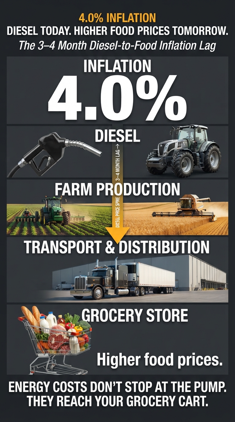
📈 4.0% INFLATION: DIESEL PRICES AND THE COMING FOOD INFLATION
With third-party calculations estimating annual consumer-price increases at 4.0%, up from 3.7% in September, monitoring diesel prices becomes particularly important when evaluating where food inflation is headed.
What you pay at the grocery store tomorrow may already be reflected in the diesel prices businesses are paying today.
Diesel is the lifeblood of the agricultural supply chain. It powers farm machinery, transports crops, moves food through processing facilities, and delivers products to grocery stores.
When diesel prices rise, the inflationary impact doesn’t stop at the fuel pump. It moves through the entire food supply chain, creating an estimated 3–4 month delay before higher operating costs work their way into consumer food prices.
🚜 Farm production 🚛 Freight and transportation 🏭 Food processing and distribution 🛒 Grocery-store prices
The economic lesson: Watch diesel prices today to understand food inflation tomorrow.
A closer look at the relationship between energy costs, agricultural production, and the inflationary pressures facing American households.
Energy prices are a major driver of food inflation. Among the most important indicators is diesel fuel, which powers the machinery, transportation networks, and logistics infrastructure supporting the entire agricultural supply chain.
Diesel price increases can provide an early warning of broader food-price inflation, with an estimated transmission lag of approximately three to four months. This delay reflects the time required for higher fuel and operating costs to move through agricultural production, freight transportation, food processing, distribution, and retail pricing.
The relationship is particularly important because food inflation does not respond to energy-price increases instantaneously. Instead, rising costs accumulate throughout the supply chain, creating a delayed inflationary effect that eventually reaches consumers.
This process resembles a supply-chain bullwhip effect: an initial increase in fuel costs propagates through multiple stages of production and distribution, amplifying operating expenses before they appear in retail food prices.
1. The October 2026 Inflation Report
The October 2026 Consumer Price Index (CPI) report released by the U.S. Bureau of Labor Statistics showed that overall consumer prices increased 0.4% month-over-month, while core inflation, which excludes volatile food and energy prices, increased 0.3%.
Third-party inflation calculations estimate that overall U.S. consumer prices are running approximately 4.0% higher than a year ago, up from an estimated 3.7% in September.
Although the October annual comparison is not an official BLS twelve-month CPI calculation, the third-party estimate provides an additional perspective on the continuing inflationary pressures affecting American households.
The distinction matters because inflation is not simply a measurement of what consumers paid last month. It reflects the cumulative increase in the cost of living, including the essential expenses of food, transportation, housing, and energy.
The relationship between energy costs and food prices deserves particular attention because changes in fuel prices can affect agricultural production and distribution well before their full impact appears in consumer inflation statistics.
2. Why Diesel Prices Lead Food Inflation
Diesel is one of the fundamental inputs supporting the modern food economy. Its influence extends across four interconnected stages of the agricultural supply chain.
A. Agricultural Production: The Farm-Level Lag
Diesel powers much of the heavy equipment required to produce food, including:
Tractors and planting equipment.
Combines and harvesting machinery.
Irrigation pumps and agricultural transport vehicles.
Equipment used for moving crops and materials around farms.
The transmission mechanism:
When diesel prices increase, farmers face higher operating costs for planting, cultivating, irrigating, and harvesting crops.
Those expenses become embedded in production costs. Depending on the crop, growing season, and timing of the fuel purchase, the increased costs may not be reflected in food prices until the resulting harvest moves through processing and distribution.
The inflationary effect: Higher agricultural production costs eventually place upward pressure on wholesale and retail food prices.
B. Freight and Logistics: The Transportation Lag
Food is particularly dependent on transportation because it must move from farms to processors, warehouses, distributors, and grocery stores.
Diesel powers much of the transportation infrastructure, including:
Commercial trucking fleets.
Agricultural freight transportation.
Diesel-powered rail locomotives.
Port equipment and certain shipping operations.
The transmission mechanism:
When diesel prices rise, trucking and logistics companies experience higher operating expenses. Fuel surcharges, freight-rate adjustments, and contract renegotiations transmit these increases to food distributors and manufacturers.
Existing transportation contracts and pricing arrangements can delay the full pass-through of higher fuel costs.
The inflationary effect: Higher freight expenses increase the delivered cost of food, creating additional upward pressure on wholesale and retail prices.
C. Food Processing, Warehousing, and Distribution
The agricultural supply chain does not end when crops leave the farm. Food must be processed, packaged, refrigerated, stored, and distributed before reaching consumers.
These operations depend on substantial energy inputs and transportation infrastructure.
The transmission mechanism:
Higher diesel prices increase the cost of moving agricultural commodities, transporting processed products, operating distribution fleets, and maintaining inventory throughout the supply chain.
Food manufacturers and retailers also operate under existing purchasing agreements and inventory cycles. They may temporarily absorb increased expenses rather than immediately passing every cost increase to consumers.
As inventories turn over and contracts are renewed, accumulated cost increases become more visible in wholesale and retail pricing.
The inflationary effect: Energy and transportation costs work their way through processing and distribution, extending the time between an initial diesel-price increase and its appearance at the grocery store.
D. Fertilizer and Agricultural Input Costs
Fuel prices also interact with the broader agricultural energy market.
Natural gas is a major feedstock for nitrogen fertilizer production, while petroleum-based inputs and diesel-powered transportation contribute to the cost of manufacturing and distributing agricultural chemicals and fertilizers.
The transmission mechanism:
Higher energy prices can increase fertilizer manufacturing, transportation, and distribution expenses. Farmers then face higher input costs when purchasing fertilizer for subsequent planting seasons.
Depending on the timing and magnitude of these increases, farmers may pay more for fertilizer, adjust application rates, or change planting decisions.
These decisions can affect production costs and, in some circumstances, crop yields during subsequent growing and harvesting cycles.
The inflationary effect: Higher agricultural input costs can contribute to additional food-price pressures months after the original energy-price increase.
3. The Three-to-Four-Month Inflation Transmission Window
The combined effects of agricultural production, transportation, processing, and distribution create a delay between changes in diesel prices and their eventual impact on consumer food prices.
The estimated three-to-four-month window represents a useful economic hypothesis for monitoring inflationary pressures. It is not a fixed delay applying equally to every food category or every fuel-price increase.
Different commodities respond at different speeds:
Fresh produce can experience relatively rapid transportation-cost pass-through.
Meat and poultry prices are influenced by feed costs, production cycles, processing, and refrigeration.
Packaged foods can experience longer delays because of inventory management, purchasing agreements, and manufacturing cycles.
The important economic principle is that energy-price increases propagate through the supply chain over time. Consequently, today’s diesel prices can provide information about potential food-price pressures in the months ahead.
4. Why This Relationship Matters for Inflation Forecasting
Traditional inflation analysis frequently concentrates on the latest CPI readings. However, CPI is a lagging indicator of many underlying production and distribution costs.
Diesel prices offer a different perspective because they reflect an important operating expense throughout the physical economy.
Monitoring diesel prices alongside food prices can help identify emerging inflationary pressures before they become fully visible in retail statistics.
A useful forecasting model would examine:
Monthly changes in national diesel prices.
Changes in agricultural production and input costs.
Changes in freight transportation costs.
Subsequent changes in wholesale food prices.
The eventual pass-through into grocery-store food prices.
Comparing these indicators over multiple years would help establish the actual transmission lag, quantify the relationship, and determine whether the three-to-four-month estimate holds consistently.
A particularly useful approach would be to compare diesel-price movements against the BLS Food at Home CPI, using time-lagged correlations and regression analysis. This would help distinguish the predictive relationship from the influence of other variables, including weather, crop yields, commodity markets, labor costs, and international supply disruptions.
5. Economic Implications
Food and energy are essential household expenses. When both experience sustained price increases, the resulting pressure on household budgets can be substantial.
Higher diesel prices affect more than what consumers pay at the pump. They increase the cost of producing, transporting, processing, and distributing the food Americans purchase every day.
This creates an important distinction between the initial inflationary shock and its downstream consequences.
Even when diesel prices stabilize, previously accumulated increases in production, freight, and distribution costs can continue working their way through the supply chain. Consequently, food inflation can remain elevated after the original fuel-price increase has subsided.
For policymakers, investors, businesses, and consumers, monitoring diesel prices provides an additional tool for evaluating future inflation risks.
Conclusion: Watch Diesel Today to Understand Food Inflation Tomorrow
Diesel is more than a transportation expense. It is a fundamental operating input throughout the agricultural economy.
Its influence extends from planting and harvesting to processing, refrigeration, transportation, warehousing, and retail distribution.
The estimated three-to-four-month transmission window illustrates why changes in diesel prices deserve attention when evaluating the future direction of food inflation.
With third-party calculations placing annual consumer-price increases at approximately 4.0%, up from 3.7% in September, the inflationary pressures affecting American households remain an important economic concern.
The broader economic lesson is straightforward:
By the time higher diesel costs appear in grocery-store prices, the inflationary pressures responsible for those increases have already been moving through the agricultural supply chain for months.
Monitoring diesel prices today provides an opportunity to anticipate tomorrow’s food inflation.
Record Global Temperatures, Converging Feedback Networks, and the Emergence of a Climate-System Singularity
By Daniel Brouse and Sidd Mukherjee
“October has continued the pattern of remarkable global warmth, with record global and surface ocean temperatures. An exceptionally strong El Niño is adding further heat to a climate already warmed by human activities, while 2026 is on track to become the second calendar year above 1.5°C. Particularly significant is that the four-year average is also expected to exceed 1.5°C, highlighting how sustained this period of global warmth has become.”
— Samantha Burgess, Strategic Lead for Climate at ECMWF
Simplified Overview
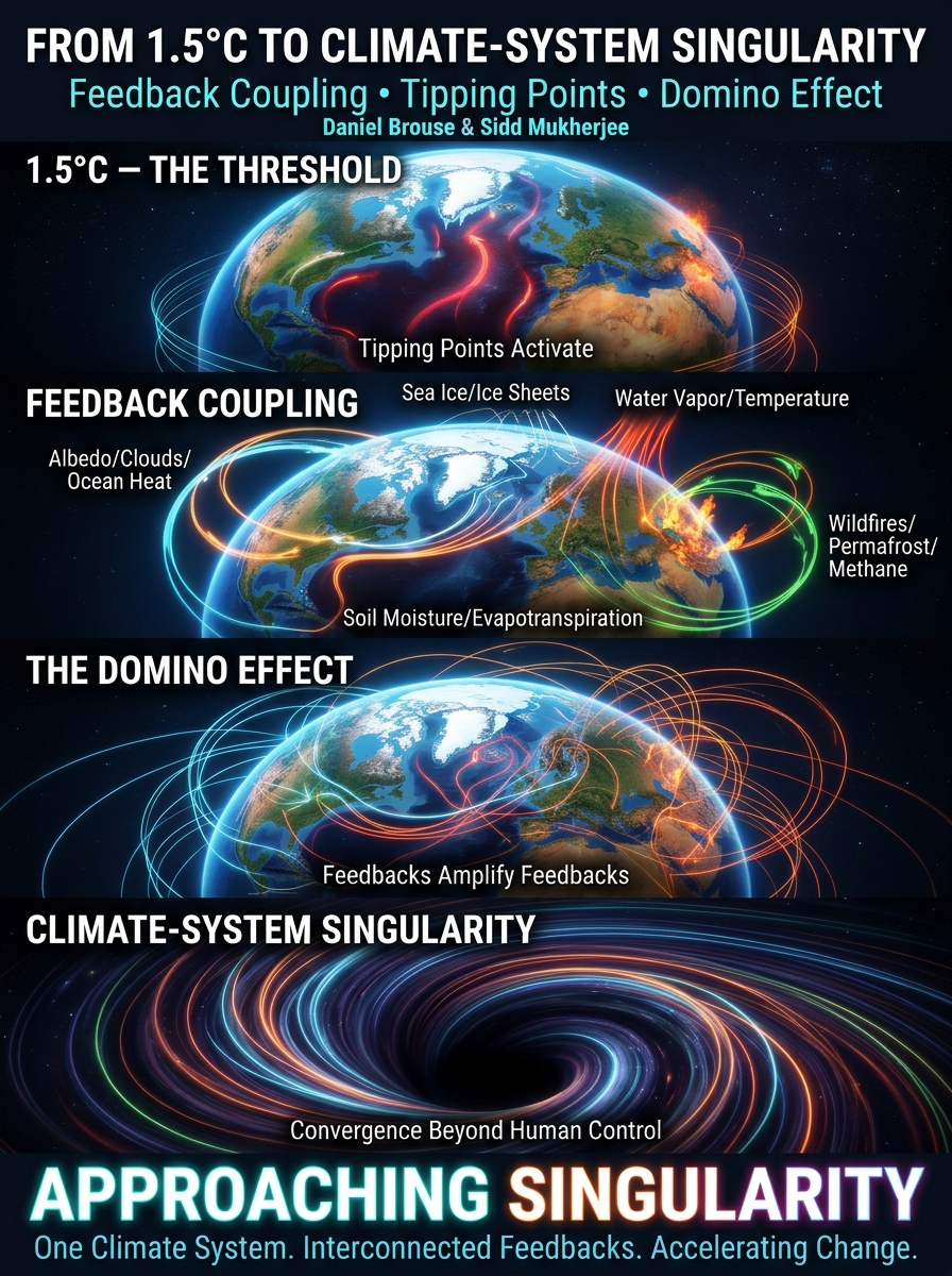
🌎 BEYOND 1.5°C: THE CLIMATE TRIPWIRE
Why is 1.5°C such an important number? And why is the accelerating pace of global warming only part of the story?
The climate system is not a thermostat. It is an interconnected network of oceans, atmosphere, ice, land, and ecosystems, with millions of interacting processes that influence one another.
As global temperatures rise, individual climate feedbacks strengthen, couple, and amplify. Ocean heat accumulation, melting ice, declining albedo, changing cloud patterns, and ecosystem deterioration are not isolated developments. They are interconnected processes capable of reinforcing one another.
The danger is not simply how much warmer Earth becomes. It is what happens as these feedbacks interact.
In our latest research paper, Daniel Brouse and Sidd Mukherjee explore the significance of the 1.5°C threshold, the convergence of climate feedback networks, and the concept of a Climate-System Singularity: a stage of increasingly interconnected, self-reinforcing planetary change that becomes progressively more difficult to predict, manage, or reverse.
We examine a fundamental question:
Are we approaching a point where the combined behavior of Earth’s climate feedback networks increasingly determines the planet’s trajectory?
1.5°C is not the destination. It is the tripwire.
And understanding what happens beyond it may be one of the most important scientific challenges of our time.
One reason the public has become so focused on this number is its simplicity. A 1.5°C (2.7°F) increase sounds like a straightforward, easily understood concept. It also doesn’t sound particularly frightening. After all, what’s the big deal about a couple of degrees of warming? Some people even portray higher temperatures as potentially beneficial.
Scientists take a very different view.
There are many ways to examine climate change. At the micro level, millions of individual feedback processes operate throughout the Earth system, connecting the atmosphere, oceans, ice, land, ecosystems, and human systems. At the macro level, these interactions combine to form one interconnected planetary climate system.
The critical question is not simply how much the planet warms, but what happens as warming changes the system itself.
Understanding how these feedbacks interact—and, more importantly, how they amplify one another—is at the frontier of climate science. The climate system is not a simple thermostat in which each additional degree produces a proportionally larger but otherwise predictable effect. It is a complex, nonlinear system capable of crossing thresholds, reorganizing feedback relationships, and shifting toward fundamentally different states.
That is why 1.5°C matters.
The 1.5°C threshold identified in the Paris Agreement, along with the approximately 2°C level associated with substantially greater climate risks, is not important because the difference between 1.4°C and 1.5°C is somehow magical. These benchmarks matter because increasing global temperatures raise the probability of activating major climate tipping elements and destabilizing interconnected Earth systems.
Once tipping processes become established, two fundamental characteristics make the consequences increasingly difficult to manage.
First, certain tipping processes can initiate self-reinforcing feedbacks that continue driving change even if the original forcing is reduced. Some changes can become effectively irreversible on human timescales.
Second, climate impacts do not necessarily increase gradually with temperature. They can accelerate, compound, and cascade as interconnected systems become destabilized and begin reinforcing one another.
Consequently, the distinction between 2°C, 3°C, or even 4°C of eventual warming cannot be understood through temperature alone. The trajectory of the Earth system, the activation of tipping elements, and the strength of interacting feedbacks become equally important.
In other words, 1.5°C is not a destination. It is not merely a warning sign or an alarm. It is a tripwire.
A warning sign tells us that danger lies ahead. An alarm tells us that danger may already be present. A tripwire represents something different: crossing a threshold that can initiate a chain of events that becomes increasingly difficult to contain, control, or reverse.
That is the critical distinction lost when climate change is reduced to a single temperature number.
The real danger lies not in the number itself, but in what the Earth system is doing as we move beyond it.
We are not simply adding another fraction of a degree to a static planet. We are increasing the energy accumulating within a dynamic, interconnected system—and that additional energy is altering the very processes that determine how the system responds.
The question, therefore, is not simply:
How many degrees warmer will Earth become?
The more important question is:
What happens as we cross the tripwires?
2. Climate-System Singularity: The Convergence of Feedback Networks
The answer requires looking beyond individual climate feedbacks and examining how they interact as interconnected networks.
Individual feedbacks do not operate in isolation. As warming intensifies, feedback processes emerge, strengthen, couple, and increasingly influence one another. These relationships form interconnected networks in which changes in one component propagate through multiple others.
Consider the relationships among:
Atmospheric warming: Increasing temperatures raise atmospheric water vapor concentrations and alter circulation patterns.
Ocean heat accumulation: The oceans absorb more than 90% of the excess energy accumulating in the Earth system, influencing ocean circulation, sea ice, and marine ecosystems.
Cryosphere destabilization: Melting sea ice reduces planetary reflectivity, while ice-sheet deterioration contributes to sea-level rise and changes in regional circulation.
Albedo changes: The loss of reflective ice and snow exposes darker surfaces that absorb more incoming solar energy.
Cloud feedbacks: Changes in cloud distribution, altitude, and properties alter the balance between incoming solar radiation and outgoing terrestrial radiation.
Ecosystem deterioration: Heat, drought, fire, and atmospheric pollution weaken vegetation and carbon sinks, changing the exchange of energy, water, and carbon between the land and atmosphere.
Each process influences other components of the system. Those interactions create additional pathways for amplification.
As these pathways multiply and strengthen, individual feedbacks increasingly become components of larger, interconnected feedback networks.
The result is a transition from isolated feedback responses toward increasingly coupled and self-reinforcing planetary processes.
We describe the potential convergence of these interacting networks as a Climate-System Singularity.
A climate-system singularity represents a critical stage in which interconnected feedback networks become increasingly self-reinforcing, driving planetary change that becomes progressively more difficult to predict, manage, or reverse through human intervention.
The concept draws an analogy to a gravitational singularity, such as the theoretical singularity associated with a black hole. It does not suggest that the climate system literally develops a gravitational singularity. Rather, it illustrates a fundamental concern: as multiple interacting forces converge, conventional assumptions about predictability, proportional responses, and human control become increasingly inadequate.
In the climate system, the concern is that feedback networks can become sufficiently interconnected and amplified that their collective behavior increasingly determines the direction and pace of planetary change.
Human emissions remain the principal external driver of contemporary global warming. However, once feedback processes become established and increasingly coupled, reducing emissions alone does not guarantee that every activated Earth-system process will immediately stop or reverse.
This distinction has profound implications for climate science, climate modeling, and public policy.
The challenge is no longer simply measuring how quickly global temperatures are rising. It is understanding how rapidly the underlying planetary systems are reorganizing, how feedback pathways are strengthening, and whether their interactions are accelerating toward cascading destabilization.
The defining question becomes whether humanity is approaching a point at which the combined behavior of Earth’s feedback networks increasingly governs the climate trajectory beyond the reach of conventional intervention.
A November 2026 Observational Assessment of Energy Accumulation, Feedback Synchronization, and Nonlinear Acceleration
By Daniel Brouse and Sidd Mukherjee
Membrane Institute — Independent Earth-System Research
Assessment date: November 10, 2026 Research period: 1970–2026 Primary common observational window: 2005–2026
Abstract
Earth’s Energy Imbalance (EEI) provides a fundamental measurement of the rate at which the Earth system accumulates energy. However, understanding the evolution of planetary energy accumulation requires examining the internal climate processes that redistribute, retain, and amplify that energy.
This paper presents an observational assessment of the proposed Earth-System Energy Imbalance–Coupled Feedback Acceleration Index (EEI–CFAI), a quantitative framework designed to investigate the relationships among planetary energy accumulation and 15 pairwise interactions involving six foundational climate variables: planetary albedo, cloud radiative effect, sea ice, atmospheric water vapor, ocean heat uptake, and global surface temperature.
The November 2026 assessment establishes that the planetary energy imbalance remains substantially elevated relative to the beginning of the satellite observational record. An independently reported CERES-derived energy imbalance tracker indicates a trailing 12-month mean of approximately 1.65 W/m² through August 2026, compared with approximately 0.43 W/m² during the first 48 months of the CERES record. The recent trailing 48-month mean is approximately 1.45 W/m².
Independent cryosphere observations also indicate substantial negative sea-ice extent anomalies. October 2026 global sea-ice extent was reported at 8.5% below the 1991–2020 average.
However, the source audit identified a significant limitation in constructing a continuous six-variable CFAI from 1970 through 2026. The specified monthly NOAA 0–2000-meter ocean heat content dataset begins in 2005, while CERES planetary radiation and cloud observations begin in 2000. Consequently, a fully consistent six-variable observational CFAI cannot be calculated across the entire proposed historical period using the specified primary datasets.
The assessment therefore establishes three distinct analytical periods: historical climate-variable context from 1970–1999, an early satellite observational period from 2000–2004, and the primary common six-variable observational period beginning in 2005.
The findings support continued investigation of the relationship between planetary energy accumulation and coupled internal climate feedbacks. They do not yet establish numerical CFAI acceleration, statistically significant feedback jerk, predictive precedence, or physical causation. Those conclusions require completion of the aligned observational calculations and statistical validation.
The Earth’s climate system is experiencing persistent planetary energy accumulation.
Earth’s Energy Imbalance measures the difference between incoming solar energy and outgoing energy escaping to space. A sustained positive imbalance means that more energy enters the Earth system than leaves it.
The accumulated energy is distributed throughout the climate system, with the oceans absorbing the overwhelming majority of the excess energy.
Understanding the evolution of EEI requires more than examining its magnitude. It also requires investigating the relationships among the internal climate variables that influence planetary reflectivity, atmospheric energy retention, ocean heat uptake, and surface temperature.
These relationships are not necessarily independent.
Declining sea ice reduces planetary reflectivity. Changes in cloud radiative effects alter the balance between reflected solar radiation and outgoing longwave radiation. Increasing atmospheric water vapor changes the atmosphere’s capacity to retain energy. Ocean heat uptake influences the distribution and storage of accumulated energy.
These processes interact.
The central research question is therefore:
Are internal climate feedback relationships becoming increasingly synchronized and amplified, and does their evolution provide measurable information about changes in planetary energy accumulation?
The EEI–CFAI framework was developed to investigate this question using observational data rather than relying exclusively on climate-model simulations.
The November 2026 refresh provides an initial observational assessment, a data-availability audit, and a revised implementation strategy for completing the six-panel analysis.
2. Research Framework
The proposed Coupled Feedback Acceleration Index incorporates six primary Earth-system variables.
2.1 Six foundational climate variables
Planetary Albedo (A): Derived from CERES top-of-atmosphere reflected shortwave radiation relative to incoming solar radiation. The orientation is inverted so declining planetary reflectivity represents a positive warming-oriented anomaly.
Cloud Feedback (C): Derived from CERES shortwave and longwave cloud radiative effects. Net cloud radiative effect is calculated as the sum of shortwave and longwave contributions, with orientation adjusted so increasing planetary energy retention is positive.
Sea Ice (S): Derived from NSIDC passive microwave satellite records. Arctic and Antarctic observations are calculated independently before aggregation. The index is inverted so declining sea-ice extent represents a positive warming-oriented anomaly.
Atmospheric Water Vapor (W): Derived from ECMWF ERA5 total-column water vapor, with independent radiosonde and satellite observations used for cross-validation.
Ocean Heat Uptake (O): Derived from the time derivative of NOAA/NCEI ocean heat content, prioritizing the 0–2000-meter inventory. Changes are converted into energy flux units for physical comparison with EEI.
Global Surface Temperature (T): Derived primarily from NASA GISTEMP, with HadCRUT5 and Berkeley Earth providing independent comparisons.
EEI remains an independent thermodynamic reference measurement. It is not included as one of the six internal variables or in the 15-pair coupling matrix.
2.2 The 15 weighted coupling relationships
The framework assigns the following weights:
Coupling relationship
Weight
Albedo × OHC
14.3%
Cloud × OHC
13.2%
Albedo × Cloud
12.1%
Sea Ice × OHC
8.0%
Water Vapor × OHC
9.0%
Water Vapor × Cloud
7.5%
Sea Ice × Albedo
7.0%
Temperature × OHC
6.0%
Temperature × Water Vapor
5.0%
Temperature × Cloud
4.5%
Sea Ice × Cloud
3.5%
Albedo × Water Vapor
3.5%
Sea Ice × Water Vapor
2.5%
Sea Ice × Temperature
2.0%
Albedo × Temperature
1.9%
Total
100.0%
The three highest-weighted relationships are:
Albedo × Ocean Heat Content: 14.3%.
Cloud × Ocean Heat Content: 13.2%.
Albedo × Cloud: 12.1%.
Together, these three pathways account for 39.6% of the proposed composite index.
These are prescribed analytical weights, not empirically established regression coefficients. Their contribution to actual observed climate behavior must be determined through calculation and sensitivity testing.
3. November 2026 Observational Findings
3.1 Earth’s Energy Imbalance
The initial observational assessment identifies a substantial increase in the reported CERES-derived EEI averages relative to the beginning of the satellite record.
The independently published CERES-derived tracker reports:
Measurement
Reported EEI
First 48 months of CERES record
+0.43 W/m²
Recent trailing 48-month mean
+1.45 W/m²
Trailing 12-month mean through August 2026
+1.65 W/m²
Highest complete calendar-year mean identified
+1.84 W/m² (2023)
The recent 48-month average is approximately 3.4 times the initial 48-month average.
These figures demonstrate that the planetary energy imbalance has remained substantially elevated during the recent observational period.
They should not be interpreted as a freshly calculated 1970–2026 EEI trend or as a measurement of the CFAI. The values are reported CERES-derived averages from an independent tracker and require direct reproduction from the underlying observational files for inclusion in a fully reproducible analysis.
The findings establish the importance of investigating whether changes in internal feedback relationships are associated with the elevated planetary energy imbalance.
3.2 Sea-Ice Observations
Independent OSI SAF observations provide additional evidence of substantial cryosphere anomalies.
October 2026 global sea-ice extent was reported at 8.5% below the 1991–2020 reference average.
The reported hemispheric anomalies were:
Arctic: 8.5% below average.
Antarctic: 9.3% below average.
These observations are relevant to the sea-ice and planetary-albedo pathways.
Declining ice extent reduces the reflective surface area of the cryosphere, increasing the potential for additional solar energy absorption.
However, sea-ice extent alone does not quantify the complete planetary albedo response. The latter must be measured using the appropriate radiation observations.
3.3 Temperature Observational Status
The source audit identified HadCRUT5 version 5.2.0.0, released September 18, 2026, with a 200-member uncertainty ensemble.
NASA GISTEMP’s September 2026 release was the latest scheduled release available on the November 10 assessment date. The October release was scheduled for November 12.
Berkeley Earth’s 2026 high-resolution dataset was identified as provisional beta material.
Accordingly, the temperature cross-validation must preserve differences in release status and uncertainty rather than treating all three datasets as equivalent finalized observations.
4. The Critical Historical Data-Coverage Limitation
One of the most important findings of the November 2026 assessment concerns the historical coverage of the six foundational variables.
The original research framework proposed a 1970–2026 analysis. However, the primary observational sources do not provide a common six-variable monthly record over that entire period.
Variable
Primary observational coverage
Historical limitation
Planetary albedo
CERES beginning March 2000
No equivalent CERES record for 1970–1999
Cloud radiative effect
CERES beginning March 2000
No consistent CERES record for 1970–1999
Sea ice
NSIDC beginning November 1978
Earlier observations unavailable in the specified record
Water vapor
ERA5 beginning 1940
Historical reanalysis rather than equivalent direct observations
Ocean heat content
NOAA monthly 0–2000 m analyzed fields beginning 2005
No equivalent specified monthly series for 1970–2004
Surface temperature
GISTEMP and HadCRUT5 beginning in the nineteenth century
Historical coverage available
This creates an important distinction between the historical research period and the common observational calculation period.
The analysis should therefore maintain three separate periods:
Period 1: 1970–1999 — Historical Climate Context
Individual historical climate observations and reconstructions can be investigated. However, a complete six-variable CFAI must not be presented as an observed result.
Period 2: 2000–2004 — Early Satellite Observational Period
CERES and NSIDC observations become available, but the specified primary NOAA 0–2000-meter monthly ocean heat content dataset remains unavailable.
Period 3: 2005–2026 — Primary Common Observational Period
All six specified variables can potentially be assembled into a common observational matrix, subject to actual monthly availability, release dates, and quality-control requirements.
The primary six-variable CFAI calculation should begin in 2005.
This adjustment preserves the historical research objective while avoiding synthetic extensions of the composite index.
5. Six-Panel Analytical Architecture
The complete EEI–CFAI visualization consists of six coordinated analytical panels.
Panel 1: Planetary Energy Imbalance
This panel establishes the independent thermodynamic reference.
It displays EEI in watts per square meter, including annual observations, smoothing curves, and the zero-energy-balance reference.
The primary analytical question is whether the planetary energy imbalance is increasing and whether its rate of change is itself changing.
Panel 2: Composite Coupled Feedback Acceleration Index
This panel displays the weighted aggregate of the 15 pairwise interactions on a 0–100 scale.
The calculation is:
CFAI(t) = 100 × Σ[w(k) × C(k,t)]
The composite should be calculated only after all six variables have been aligned, standardized, and quality controlled.
The 2005–2026 common observational period is the primary calculation window.
Panel 3: Feedback Velocity, Acceleration, and Climate Jerk
The three derivatives provide distinct measures of the changing feedback system.
Velocity:
v(t) = dCFAI/dt
Acceleration:
a(t) = d²CFAI/dt²
Climate jerk:
j(t) = d³CFAI/dt³
These measurements distinguish increasing feedback intensity from increasing feedback acceleration.
A positive third derivative indicates increasing acceleration, not necessarily a permanently accelerating climate system.
The calculations must include uncertainty estimates and smoothing sensitivity.
Panel 4: Fifteen Coupling Pathways
This panel uses a heatmap to show the changing intensity of all 15 interactions.
A second heatmap displays each pathway’s weighted contribution to the aggregate CFAI.
This distinction is important because the strongest individual coupling is not necessarily the strongest contributor to the composite index.
Panel 5: Feedback Lead–Lag Relationships
This panel investigates whether changes in internal feedback relationships precede changes in EEI.
The analysis covers immediate, short-term, intermediate, multiyear, and longer-term relationships.
Cross-correlation and distributed-lag regression are required.
The lag sign convention must be explicitly documented.
Granger-predictive testing can establish whether earlier CFAI observations provide additional predictive information about subsequent EEI observations. It cannot independently establish physical causation.
Panel 6: EEI–CFAI Synchronization
The final panel compares the two independent measurements.
It includes:
Annual EEI and CFAI trajectories.
Contemporaneous correlation.
First-differenced correlation.
Detrended residual analysis.
Lagged regression coefficients.
Confidence intervals and uncertainty estimates.
The central question is whether changes in internal feedback coupling correspond to changes in planetary energy accumulation and whether the former provide measurable predictive information about the latter.
6. Statistical Validation Requirements
The framework requires several statistical safeguards before its numerical results can support conclusions about nonlinear acceleration.
This reduces the influence of extreme observations on standardization.
6.2 Co-Amplification
For each pair of warming-oriented standardized variables:
P(i,j,t) = max(0,Z(i,t)) × max(0,Z(j,t))
The bounded co-amplification measure is:
M(i,j,t) = tanh[P(i,j,t)/2]
6.3 Statistical Coupling
The framework incorporates rolling partial correlation:
R(i,j,t) = max(0, ρ(i,j|X))
The external control variables include ENSO, volcanic stratospheric aerosol optical depth, solar irradiance, and anthropogenic aerosol forcing changes.
The composite pairwise coupling function is:
C(i,j,t) = 0.5M(i,j,t) + 0.5R(i,j,t)
The 50/50 weighting should be tested against 40/60 and 60/40 alternatives.
6.4 Smoothing Sensitivity
Annual averages should be evaluated using centered Savitzky–Golay filters with:
9-year window.
11-year window.
15-year window.
The 11-year filter remains the primary specification.
Endpoint estimates must be marked provisional because centered filtering cannot provide equivalent historical context beyond the available observations.
Benjamini–Hochberg false-discovery-rate control at q = 0.05.
At least 5,000 block-bootstrap iterations.
Confidence intervals for composite values and derivatives.
Detrended and first-differenced correlation tests.
Lagged predictive regression and Granger-predictive testing.
These procedures have not yet been completed for the November 2026 refresh.
7. Limitations and Outstanding Calculations
The November 2026 assessment is an observational source audit and preliminary energy-imbalance assessment. It is not a completed numerical CFAI analysis.
The following results remain outstanding:
Monthly aligned observations for all six variables.
Numerical calculations for all 15 pairwise coupling scores.
The complete 2005–2026 composite CFAI.
CFAI velocity, acceleration, and jerk.
Bootstrap confidence intervals.
Serial-correlation-corrected trend results.
False-discovery-rate-adjusted significance.
Lead–lag correlation matrices.
Distributed-lag regression.
Granger-predictive testing.
EEI–CFAI synchronization statistics.
Additional implementation decisions are required concerning rolling partial-correlation window length, external-control estimation, and the treatment of changes in observational systems.
The ocean heat uptake variable also requires particular care. Ocean heat content is accumulated energy, while ocean heat uptake is its rate of change. The CFAI must use the latter, expressed as an energy flux, rather than inadvertently mixing accumulated heat content with a monthly rate.
These limitations are not evidence against the proposed framework. They identify the work required to turn the framework into a reproducible observational index.
8. Conclusions
The November 2026 observational assessment establishes that Earth’s planetary energy imbalance remains substantially elevated relative to the beginning of the CERES observational record.
The reported trailing 12-month mean through August 2026 was approximately 1.65 W/m², compared with approximately 0.43 W/m² during the first 48 months of the CERES record.
Independent October 2026 observations also document substantial sea-ice extent anomalies in both hemispheres.
Together, these observations reinforce the importance of investigating the relationships between planetary energy accumulation and the internal climate processes that influence energy retention and redistribution.
The proposed EEI–CFAI framework provides a structured method for investigating those relationships through 15 weighted interactions involving six foundational climate variables.
The most important methodological finding is that the primary common six-variable observational window begins in 2005, rather than 1970. The longer historical period remains useful for examining individual climate variables and broader Earth-system developments, but it cannot be represented as a continuous six-variable CFAI without introducing alternative historical datasets and explicitly documenting their limitations.
The next stage of research is to calculate the complete common-period index, evaluate its derivatives, identify the dominant coupling pathways, and determine whether internal feedback synchronization provides statistically significant predictive information about EEI.
The ultimate objective is to establish whether the changing behavior of Earth’s internal climate feedback network is measurably associated with the changing rate of planetary energy accumulation.
The distinction between increasing energy accumulation, increasing feedback intensity, and nonlinear feedback acceleration must remain central to the analysis.
Each is a different physical and statistical proposition. Each requires independent observational verification.
The EEI–CFAI framework is designed to test those propositions quantitatively.
9. Primary Data Sources and Research Resources
NASA CERES — Earth radiation budget, planetary albedo, and cloud radiative effects.
National Snow and Ice Data Center — Sea Ice Index and passive microwave observations.
ECMWF — ERA5 atmospheric reanalysis and total-column water vapor.
NOAA/NCEI — Ocean heat content, 0–700 m and 0–2000 m.
NASA GISS — GISTEMP global surface temperature.
Met Office Hadley Centre — HadCRUT5 global temperature observations and uncertainty ensembles.
Berkeley Earth — Independent global temperature observations.
OSI SAF — Independent satellite sea-ice observations.
10. Research Status and Attribution
Research framework: Daniel Brouse and Sidd Mukherjee.
Assessment: November 10, 2026.
Status: Preliminary observational assessment; full numerical CFAI validation pending.
Research principle: Observational measurements, reconstructed historical records, statistical estimates, and scientific interpretations must remain separately identifiable.
The authors’ objective is to develop a reproducible, observationally grounded method for measuring Earth-system energy accumulation, internal feedback coupling, and nonlinear climate-system dynamics.
🌎 One Planet, One Climate System: How Pacific Warming Connects to a Northeast Nor’easter
A developing late-week nor’easter is forecast to bring a dramatic temperature drop, heavy rain, strong coastal winds, and the season’s first accumulating snowfall to higher elevations across the Northeast and Mid-Atlantic.
But there is a much bigger climate story unfolding behind these regional weather patterns.
The climate system is not a collection of isolated oceans, atmospheric currents, and regional weather events. It is a planetary network of interconnected energy transfers, atmospheric circulation, ocean responses, and feedbacks.
This is planetary climate-energy teleconnection.
🌊 FROM THE PACIFIC TO THE ATLANTIC
The developing super El Niño is changing the distribution of oceanic heat and atmospheric convection across the tropical Pacific.
These changes reorganize the Walker circulation, shifting atmospheric heating, pressure gradients, and wind patterns.
The resulting atmospheric bridge can extend across ocean basins:
Pacific El Niño ↓ Rerouted Walker circulation ↓ Changes in planetary atmospheric circulation ↓ Atlantic pressure and trade-wind responses ↓ Ocean circulation and temperature redistribution ↓ North Atlantic circulation and jet-stream changes ↓ Regional weather consequences across North America and Europe
The important distinction is that these connections are not isolated cause-and-effect events. They are interacting components of a planetary climate system.
🌬️ HOW THIS CONNECTS TO THE NOR’EASTER
The North Atlantic circulation, jet stream, and associated pressure systems influence the movement of storm systems and the transport of heat and moisture across eastern North America.
As atmospheric circulation patterns respond to changing tropical and oceanic conditions, the probability of particular weather regimes can change.
The developing nor’easter provides a regional example of the weather consequences we need to examine within this broader interconnected system.
Expected regional impacts:
• Philadelphia, Washington, D.C., and New York City: Cold, soaking rain rather than accumulating snow.
• Coastal areas from North Carolina to New England: Strong winds potentially exceeding 40 mph and minor coastal flooding during high tides.
• Inland mountains: The greatest potential for accumulating snowfall across northern New England, upstate New York, central Pennsylvania, and northwestern New Jersey.
• Great Lakes: Colder incoming air interacting with relatively warm lake waters, producing localized lake-effect rain and snow.
❄️ THE ENERGY CONNECTION
What makes this particularly interesting is the redistribution of energy throughout the climate system.
Ocean temperatures influence atmospheric convection. Atmospheric circulation redistributes heat and moisture. Changes in pressure and winds influence ocean circulation and upwelling. Ocean temperatures then feed back into atmospheric conditions.
These processes operate across different distances and timescales, connecting weather patterns thousands of miles apart.
The Atlantic Meridional Overturning Circulation (AMOC), North Atlantic temperature patterns, ENSO, and atmospheric wave propagation are all important components of this interconnected system. Their individual contributions must be evaluated rather than assuming that one circulation change directly produces a particular storm.
ONE PLANET. ONE INTERCONNECTED CLIMATE SYSTEM.
The question is no longer simply what weather is coming to our neighborhood.
It is how changing planetary energy distributions are influencing atmospheric circulation, oceanic responses, regional weather, and the feedback networks connecting them.
The Pacific warms. The atmosphere responds. The Atlantic adjusts. The jet stream redistributes weather patterns. Regional consequences emerge.
Energy moves through the connections. Feedbacks propagate. The planet responds.
From 1.5°C Warming to Feedback Coupling, Tipping Points, and the Domino Effect
Earth’s climate system is entering a new phase. As global warming exceeds critical thresholds, climate feedbacks increasingly interact, reinforce one another, and trigger cascading changes across the planet.
The Emerging Progression
🌡️ 1.5°C Warming → Increasing pressure on planetary tipping points.
🔄 Feedback Coupling → Climate processes begin reinforcing one another.
🧊 Tipping Points → Ice sheets, oceans, forests, and other systems become increasingly unstable.
🌪️ Domino Effect → Interconnected feedbacks amplify changes across the Earth system.
Climate change is no longer just about rising temperatures. It is about an increasingly interconnected system in which one change amplifies another.
📖 Explore the paper, examine the emerging feedback connections, and discover the scientific sources and research behind this framework.
Feedback Coupling, Tipping Points, and the Domino Effect
1. The 1.5°C Threshold: Tipping Points Activate
The 2023–2026 four-year average is projected to surpass 1.5°C above preindustrial levels. This is no longer simply a projection of future warming. We are observing the consequences of an increasingly interconnected climate feedback system in real time.
3. Climate-System Singularity: Convergence of Feedback Networks
As individual feedbacks emerge, couple, and organize into self-reinforcing networks, those networks increasingly interact and converge toward a unified, interconnected climate system.
A climate-system singularity represents a critical tipping point where interacting feedbacks drive increasingly uncontrollable and irreversible planetary change. It is analogous to a gravitational singularity, such as a black hole, where converging forces produce a point beyond which conventional predictions and control break down. In the climate system, this represents a trajectory toward increasingly unpredictable, self-reinforcing change that becomes progressively decoupled from human policy intervention.
1. IPCC (2021) — Climate Change 2021: The Physical Science Basis, Chapter 7: Earth’s Energy Budget, Climate Feedbacks, and Climate Sensitivity. Covers water vapor, clouds, surface albedo, and interconnected climate feedback processes. IPCC Chapter 7
2. IPCC (2023) — Climate Change 2023: Synthesis Report. Documents increasing risks of abrupt and irreversible climate changes, including tipping-point risks between 1.5°C and 2.5°C. IPCC Synthesis Report
3. Global Tipping Points Report (2025). Comprehensive scientific assessment of interacting Earth-system tipping elements and cascading risks. 2025 Report and downloads
4. Nature Geoscience (2025) — Destabilization of Earth System Tipping Elements. Examines interactions among Greenland, Antarctic, AMOC, and Amazon tipping elements. Read scientific paper
5. IPCC (2021) — Chapter 5: Global Carbon and Other Biogeochemical Cycles and Feedbacks. Covers permafrost, vegetation, soil carbon, ocean carbon exchange, and greenhouse gas feedbacks. IPCC Chapter 5
6. WMO (2026) — Global Annual to Decadal Climate Update 2026–2035. Provides current temperature projections and the probability of temporarily exceeding 1.5°C. WMO Climate Update
Additional research and original work
7. Daniel Brouse and Sidd Mukherjee — Climate Feedback and Tipping-Point Network. Original research
8. Daniel Brouse and Sidd Mukherjee — Observable Climate Feedback Coupling. Original research
Research Focus: Nonlinear Climate Dynamics, Feedback Coupling, and Earth-System Energy Redistribution
A Comparative Assessment of Ocean Heat Content, Albedo, Clouds, Atmospheric Water Vapor, Soil Moisture, and Emerging Carbon-Release Feedback Networks
Simplified Overview
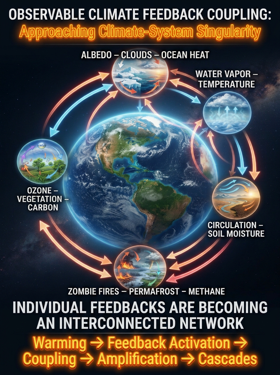
🌎 Observable Climate Feedback Coupling — The Emergence of an Interconnected Earth-System Network
Climate change is no longer adequately described by examining individual feedback loops in isolation. The increasingly interconnected behavior of Earth’s climate systems demands a broader perspective.
This paper examines five major feedback networks showing observable interactions:
The central finding is that these processes cannot be understood independently. Their interactions connect atmospheric, oceanic, terrestrial, and cryospheric systems into increasingly complex feedback networks.
Three areas deserve particularly close attention: the Albedo–Cloud–Ocean Heat triad, Water Vapor–Temperature coupling, and Circulation–Soil Moisture–Temperature interactions.
The critical question is no longer simply whether individual feedbacks are occurring. It is whether their interactions are becoming increasingly interconnected, persistent, synchronized, and mutually reinforcing.
Climate change is increasingly characterized by interactions among multiple physical, chemical, biological, and atmospheric processes. Individual climate indicators are no longer sufficient to describe the evolving behavior of the Earth system. The increasingly interconnected relationships among ocean heat content, surface albedo, low-level cloud cover, atmospheric water vapor, soil moisture, atmospheric circulation, vegetation, permafrost, and greenhouse-gas emissions provide observable evidence of expanding feedback coupling.
This paper examines the principal climate indicators demonstrating observable feedback interactions and evaluates their significance according to three criteria: the magnitude and persistence of observed changes, the number of interconnected climate processes, and the degree to which those interactions reinforce additional warming.
Five major feedback domains receive particular attention:
The analysis identifies ocean heat content, surface albedo, low-level cloud behavior, atmospheric water vapor, and soil moisture as particularly important observational indicators. It also identifies the growing interaction among terrestrial carbon release, permafrost degradation, wildfire activity, and atmospheric greenhouse-gas accumulation as an important emerging feedback network.
The central conclusion is that climate feedback research must move beyond isolated indicators and individual feedback loops. The increasing interaction, synchronization, and reinforcement of multiple climate processes require a network-based approach to monitoring Earth-system behavior.
1. Introduction: From Individual Feedbacks to Network Coupling
Traditional climate analysis frequently examines individual feedback mechanisms independently. Examples include the water vapor feedback, ice-albedo feedback, cloud feedback, and terrestrial carbon feedback.
Although these mechanisms remain scientifically important, examining them independently does not adequately characterize the increasingly interconnected behavior of the climate system.
Climate feedback coupling occurs when changes in one physical process influence another process, which subsequently reinforces or modifies the original disturbance. As these relationships become interconnected, individual feedback mechanisms form larger networks capable of amplifying changes across multiple Earth-system domains.
This framework emphasizes that the significance of climate change is not determined solely by the magnitude of an individual indicator. The interaction among indicators determines how disturbances propagate and influence other components of the Earth system.
A comprehensive observational framework must therefore evaluate:
The magnitude and direction of individual indicator changes.
The strength and persistence of relationships between indicators.
The directionality of physical interactions.
The emergence of reinforcing feedback pathways.
The development of increasingly interconnected feedback networks.
The objective is to identify which climate indicators currently provide the clearest observable evidence of this evolving behavior.
2. Criteria for Evaluating Observable Feedback Coupling
The indicators examined in this paper are evaluated using three principal criteria.
2.1 Magnitude and Persistence of Observed Change
The first criterion examines whether an indicator demonstrates measurable, persistent changes over time.
Examples include:
Increasing ocean heat content.
Declining Arctic sea-ice extent.
Changes in surface reflectivity.
Increasing atmospheric water vapor.
Declining soil moisture in vulnerable regions.
Increasing greenhouse-gas concentrations.
Persistent changes provide the observational foundation for identifying evolving climate feedback relationships.
2.2 Network Connectivity
The second criterion evaluates how many other climate processes interact with a particular indicator.
Ocean heat content, for example, connects atmospheric energy imbalance, sea-surface temperature, ocean stratification, sea-ice loss, ice-sheet melting, and ocean circulation.
Atmospheric water vapor connects temperature, evaporation, precipitation, cloud formation, and atmospheric radiation.
Indicators with numerous physical connections are especially important when evaluating the development of interconnected feedback networks.
2.3 Reinforcement and Amplification
The third criterion examines whether interactions reinforce the original disturbance.
A reinforcing feedback occurs when an initial change produces additional changes that strengthen the original effect.
For example:
Temperature increase → Increased atmospheric water vapor → Increased absorption of outgoing infrared radiation → Additional warming.
The distinction between simple correlation and actual feedback amplification is essential. Observing two indicators changing simultaneously does not independently establish a causal feedback relationship.
3. Principal Climate Indicators Demonstrating Observable Coupling
The following ranking reflects observational importance and network connectivity. It is not a quantitative ranking of total global radiative forcing or a statistically established ranking of feedback strength.
3.1 Ocean Heat Content: The Central Energy Redistribution Indicator
Ocean heat content (OHC) is one of the most important indicators of the changing Earth-system energy balance.
More than 90% of the excess energy accumulating in the Earth system is absorbed by the oceans. Consequently, ocean heat content provides a particularly important measure of continuing planetary energy accumulation.
Its principal connections include:
Atmospheric energy imbalance.
Sea-surface temperature.
Ocean stratification.
Marine heatwaves.
Sea-ice loss.
Ice-sheet and glacier melting.
Ocean circulation.
Atmospheric moisture and evaporation.
Increasing ocean heat content influences both atmospheric and cryospheric processes. It also contributes to the redistribution of energy through ocean circulation and changes in the vertical structure of the ocean.
OHC is therefore not simply another warming indicator. It is a central connecting variable in the broader climate feedback network.
3.2 Surface Albedo: The Ice-Loss Amplification Mechanism
Surface albedo measures the proportion of incoming solar radiation reflected by the Earth’s surface.
Snow and ice have relatively high reflectivity. When they disappear, darker ocean and land surfaces become exposed, increasing the absorption of incoming solar energy.
The principal reinforcing pathway is:
Warming → Snow and Ice Loss → Reduced Surface Albedo → Increased Solar Absorption → Additional Warming
This mechanism connects:
Arctic sea-ice retreat.
Antarctic sea-ice variability.
Greenland ice-sheet melting.
Mountain glacier retreat.
Snow-cover changes.
Surface temperature.
Ocean heat accumulation.
Albedo is especially important because it provides a direct physical connection between cryospheric changes and the planetary energy balance.
Its interactions with cloud cover and ocean heat content make it a particularly important indicator in higher-order feedback analysis.
3.3 Low-Level Clouds: An Important and Evolving Climate Feedback
Low-level clouds influence the Earth’s energy balance through their reflection of incoming solar radiation and their absorption and emission of infrared radiation.
Their net climate effect depends on cloud altitude, thickness, optical properties, geographical distribution, and atmospheric conditions.
Changes in low-level cloud cover can alter the amount of solar energy absorbed by the ocean and land.
The principal interactions include:
Cloud cover and surface albedo.
Cloud cover and ocean heat content.
Cloud cover and atmospheric water vapor.
Cloud cover and atmospheric circulation.
Cloud cover and surface temperature.
Declining low-cloud cover in some regions increases incoming solar energy at the surface. However, observed cloud trends are geographically and temporally variable, and increases in cloud cover can produce different radiative effects depending on cloud properties.
Consequently, low-level clouds should be treated as a major emerging feedback indicator, with regional and seasonal behavior evaluated separately.
The distinction between shortwave and longwave cloud-radiative effects is particularly important.
3.4 Atmospheric Water Vapor: A Fundamental Atmospheric Amplifier
Water vapor is the most abundant greenhouse gas and one of the most important climate feedback mechanisms.
As atmospheric temperatures increase, the atmosphere can contain more water vapor. Increased atmospheric moisture strengthens the absorption of outgoing infrared radiation, reinforcing warming.
The principal feedback sequence is:
Temperature Increase → Increased Atmospheric Water Vapor → Increased Infrared Absorption → Additional Warming
Water vapor also connects several other climate processes:
Ocean evaporation.
Land-surface evaporation.
Atmospheric rivers.
Cloud formation.
Precipitation extremes.
Atmospheric circulation.
Ice-sheet surface melting.
Its importance extends beyond its direct greenhouse effect. Water vapor is a major connecting mechanism between the atmosphere, oceans, hydrological cycle, and cryosphere.
Monitoring atmospheric moisture alongside temperature, outgoing longwave radiation, cloud properties, and precipitation provides a more complete assessment of atmospheric feedback coupling.
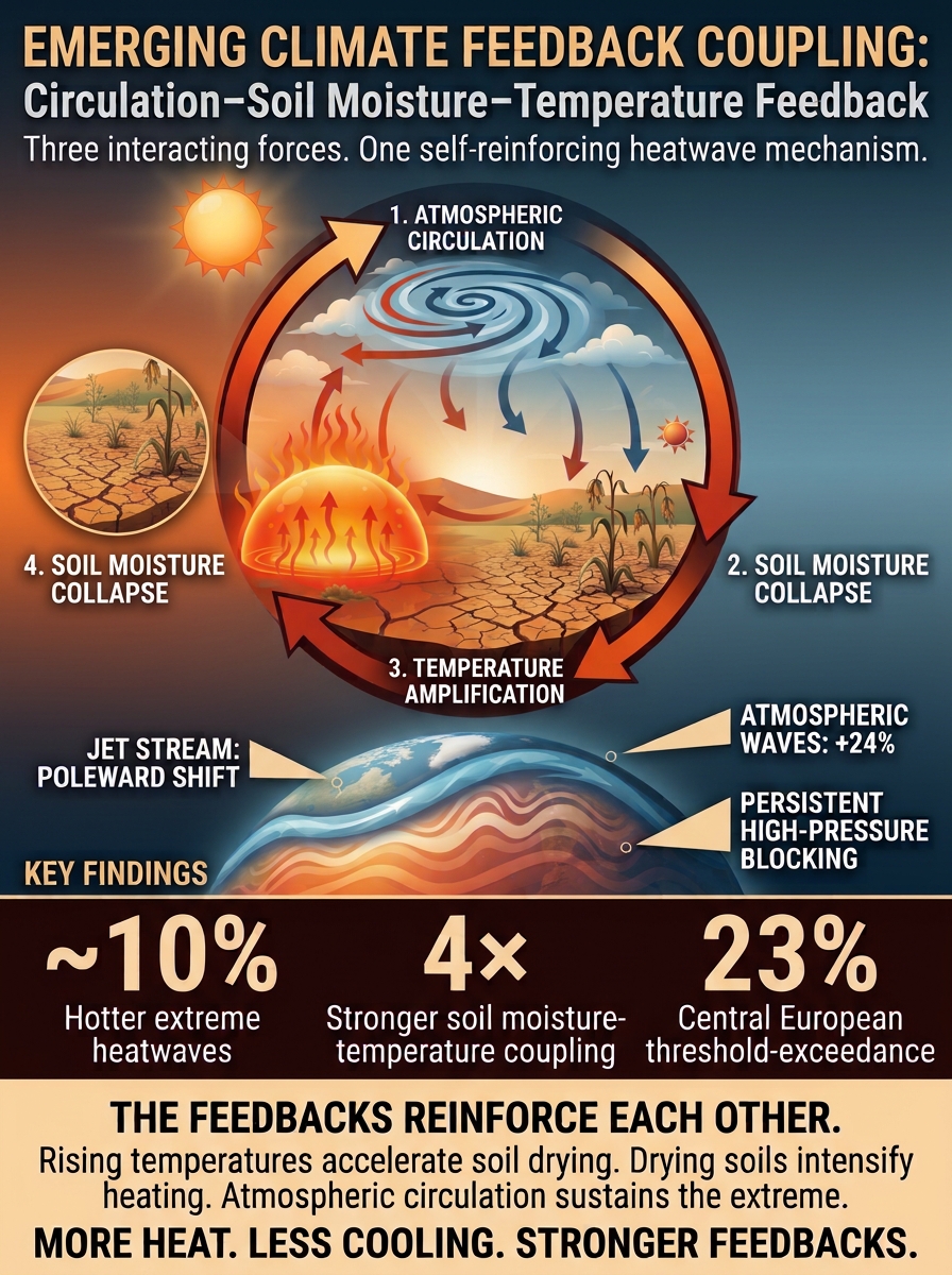
3.5 Soil Moisture and Evapotranspiration: Land–Atmosphere Feedback Coupling
Soil moisture regulates the partitioning of available surface energy between latent and sensible heat.
When sufficient soil moisture is available, evaporation and plant transpiration provide evaporative cooling.
When soil moisture declines, evaporative cooling becomes restricted and a greater proportion of available energy contributes to sensible heating.
The significance of this feedback is particularly evident during persistent heat and drought conditions.
Soil moisture is therefore an essential indicator for evaluating regional feedback amplification and the interaction between atmospheric circulation and land-surface energy redistribution.
3.6 Vegetation and Terrestrial Carbon Uptake
Vegetation provides a major natural mechanism for removing carbon dioxide from the atmosphere.
However, increasing heat stress, drought, wildfire, and ozone exposure damage vegetation and interfere with photosynthesis, stomatal function, and carbon uptake.
This feedback domain is particularly important because atmospheric chemistry, biological processes, hydrology, and climate dynamics interact directly.
Vegetation condition and carbon uptake should therefore be monitored alongside atmospheric CO₂, ozone concentrations, soil moisture, and temperature.
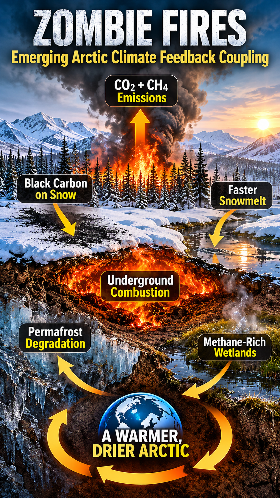
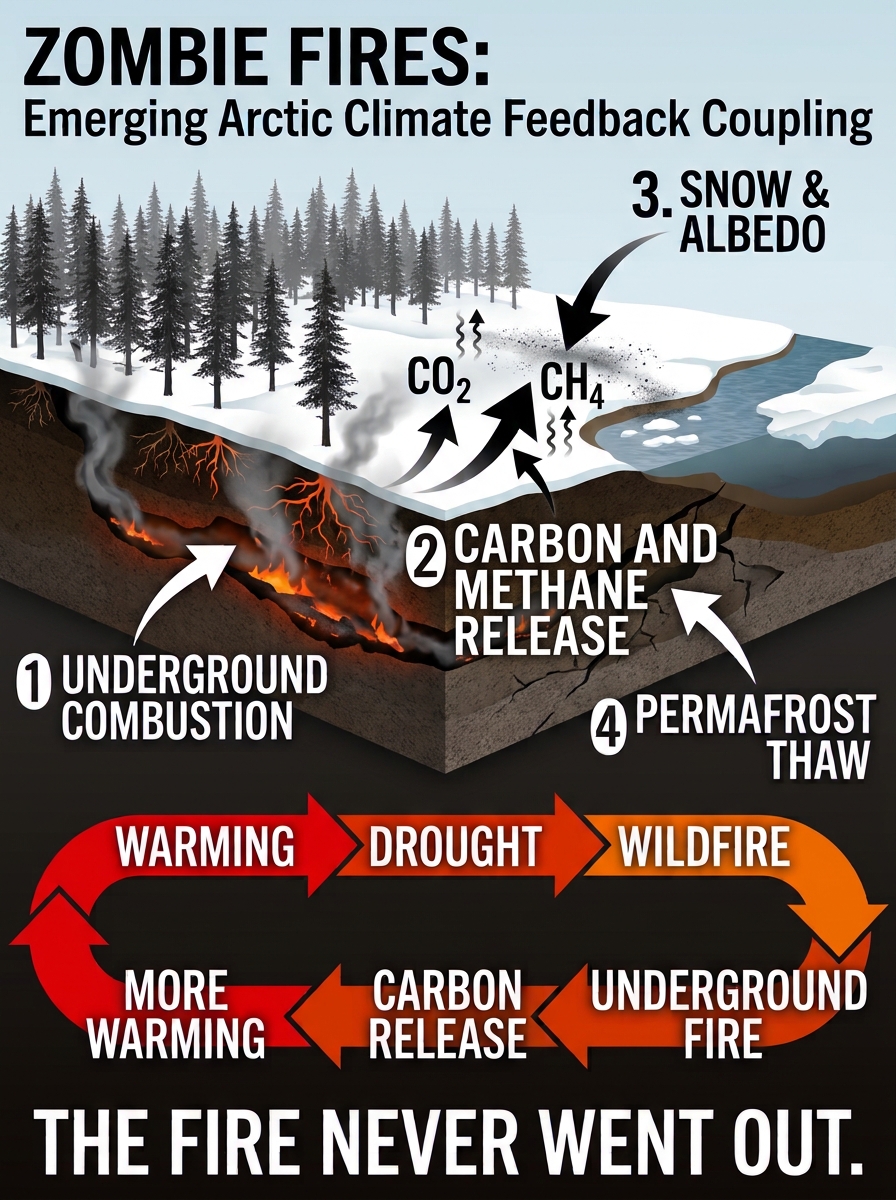
3.7 Permafrost, Wildfire, and Methane: Emerging Carbon-Release Coupling
Permafrost contains substantial quantities of previously frozen organic carbon.
As permafrost thaws, microbial decomposition releases greenhouse gases, including carbon dioxide and methane.
Wildfire activity introduces additional pathways by consuming insulating vegetation and organic soil layers, exposing previously protected carbon, and increasing the vulnerability of underlying permafrost.
The principal feedback network is:
Warming → Permafrost Thaw and Wildfire → Organic Carbon Release → CO₂ and CH₄ Accumulation → Additional Warming
Additional interactions include:
Peat combustion.
Persistent underground fires.
Vegetation loss.
Black-carbon deposition.
Snow and ice albedo reduction.
Deeper seasonal thaw.
Changes in soil hydrology.
The emerging zombie-fire feedback network is particularly important because it connects terrestrial combustion, atmospheric greenhouse-gas accumulation, permafrost degradation, and cryospheric changes.
This is an example of how previously distinct climate feedback domains become interconnected through shared physical mechanisms.
4. The Five Most Important Observable Feedback Networks
Individual indicators become more meaningful when examined through their physical relationships.
Five networks deserve particular attention.
4.1 Albedo–Cloud–Ocean Heat Content
This network connects three important components of the planetary energy balance.
Reduced surface albedo increases solar absorption. Changes in low-level cloud cover alter the amount of incoming solar radiation reflected back into space. Increased ocean heat content records the resulting accumulation of energy, together with the contributions of other energy-imbalance processes.
The three principal pairwise relationships are:
Albedo × Ocean Heat Content.
Cloud Cover × Ocean Heat Content.
Albedo × Cloud Cover.
Together, these relationships form a higher-order feedback network.
In the previously developed Coupled Climate Feedback Index, the analytical weighting assigned to these relationships was:
Relationship
Analytical weight
Albedo × OHC
14.3%
Cloud × OHC
13.2%
Albedo × Cloud
12.1%
Combined triad
39.6%
These figures represent weights within that analytical framework, not independently measured percentages of global climate forcing or proof of causal contribution.
The triad nevertheless provides a useful starting point for investigating interactions among surface reflectivity, atmospheric radiation, and planetary energy accumulation.
4.2 Ocean Heat–Cryosphere–Sea-Level Coupling
Ocean heat accumulation contributes to changes in marine and cryospheric conditions.
Increasing subsurface ocean temperatures expose vulnerable ice shelves and glacier systems to additional heat, contributing to basal melting and changes in ice discharge.
Freshwater input also changes ocean stratification and circulation, potentially altering the distribution of heat within the ocean.
This network is particularly important because it connects a relatively well-observed global indicator, ocean heat content, with major changes in the cryosphere.
This relationship deserves greater attention in climate feedback monitoring because greenhouse-gas concentrations alone do not reveal changes in the effectiveness of natural carbon sinks.
4.5 Zombie Fires–Permafrost–Carbon–Methane
Persistent peat and underground fires connect wildfire activity with permafrost degradation and greenhouse-gas release.
Combustion releases stored carbon, removes insulating vegetation and organic material, and increases exposure of underlying soils to warming.
Permafrost thaw subsequently exposes additional organic carbon to decomposition.
The resulting network connects:
Wildfire and peat combustion.
Permafrost thaw.
CO₂ emissions.
Methane emissions.
Black-carbon deposition.
Reduced surface albedo.
Additional atmospheric warming.
This network illustrates how terrestrial feedback processes can interact with atmospheric and cryospheric feedbacks.
5. A Proposed Observational Monitoring Framework
A more comprehensive approach to climate feedback research should distinguish three levels of observation and analysis.
Level 1: Directly Observable Climate Indicators
The first level measures the physical variables themselves.
Indicator
Principal measurements
Ocean heat content
Integrated ocean heat accumulation
Surface albedo
Surface reflectivity and absorbed solar radiation
Low-level clouds
Cloud fraction, optical depth, and radiative effects
Atmospheric water vapor
Specific humidity and column-integrated water vapor
Soil moisture
Surface and subsurface moisture
Evapotranspiration
Latent heat flux and vegetation transpiration
Atmospheric circulation
Winds, pressure patterns, and circulation indices
Vegetation
Productivity, photosynthesis, and carbon uptake
Permafrost
Ground temperature, active-layer depth, and thaw
Greenhouse gases
Atmospheric CO₂ and CH₄ concentrations
Earth Energy Imbalance should be included as an overarching measurement of whether the planet is accumulating or losing energy.
Level 2: Pairwise Feedback Coupling
The second level evaluates relationships between individual indicators.
Priority relationships include:
Albedo × Ocean Heat Content.
Cloud Cover × Ocean Heat Content.
Albedo × Cloud Cover.
Water Vapor × Temperature.
Soil Moisture × Temperature.
Evapotranspiration × Atmospheric Circulation.
Ozone × Vegetation Productivity.
Permafrost Thaw × Methane.
Wildfire × Carbon Release.
Sea-Ice Loss × Ocean Heat.
These relationships should be evaluated using consistent observational periods, appropriate regional and seasonal controls, lagged relationships, and physically meaningful directional tests.
Level 3: Higher-Order Feedback Networks
The third level evaluates interactions among three or more indicators.
The priority networks are:
Albedo–Cloud–Ocean Heat Content.
Ocean Heat–Cryosphere–Sea-Level.
Circulation–Soil Moisture–Temperature.
Ozone–Vegetation–Carbon Sink.
Zombie Fire–Permafrost–Carbon–Methane.
Atmospheric River–Foehn Wind–Ice-Shelf and Ice-Sheet Loss.
The objective is to determine whether individual feedback processes are becoming increasingly interconnected, persistent, and mutually reinforcing.
6. Methodological Requirements: Distinguishing Correlation from Feedback
A central requirement of this framework is distinguishing observable association from demonstrated physical feedback.
Correlation between two climate indicators does not independently establish causation, directionality, or amplification.
A rigorous assessment should therefore incorporate:
Temporal analysis: Determine whether changes occur simultaneously or whether one indicator consistently precedes another.
Directional analysis: Evaluate whether changes in one variable physically influence the subsequent behavior of another.
Physical mechanisms: Establish whether the observed relationship is consistent with known energy, mass, chemical, and biological processes.
Regional differentiation: Preserve geographical and seasonal differences rather than relying exclusively on global averages.
Lagged relationships: Evaluate whether feedback interactions develop over different timescales.
Independent validation: Compare results across observational datasets and independent analytical approaches.
Network amplification: Determine whether interactions among multiple indicators produce measurable reinforcement beyond the behavior of individual processes.
These requirements are especially important for cloud feedbacks, where the net effect depends on cloud altitude, optical properties, geographical distribution, and shortwave versus longwave radiation.
They also apply to ocean–atmosphere and land–atmosphere interactions, where internal variability and external forcing can produce correlated changes without necessarily demonstrating a reinforcing feedback.
7. Implications for the Coupled Climate Feedback Index
The Coupled Climate Feedback Index should evolve beyond measuring individual pairwise relationships.
A more comprehensive framework should incorporate:
Indicator trends and rates of change.
Pairwise coupling strength.
Directional relationships and temporal lags.
Higher-order interactions.
Persistence of reinforcing pathways.
Changes in network connectivity.
Acceleration in the development of interconnected feedbacks.
The existing Albedo–Cloud–OHC triad provides a useful foundation.
However, atmospheric water vapor, soil moisture, atmospheric circulation, vegetation condition, and carbon-release processes should also be incorporated.
A particularly useful distinction is between the magnitude of an individual indicator and its network importance.
For example, ocean heat content may demonstrate a large and persistent physical change, while atmospheric water vapor may have particularly extensive connections to other climate processes.
Similarly, soil moisture can become a dominant regional amplifier during persistent drought and heat events without necessarily representing the largest global climate forcing.
A multidimensional index should preserve these distinctions rather than collapsing all indicators into one undifferentiated score.
8. Conclusions: The Emergence of an Interconnected Climate Feedback Network
The most important development in contemporary climate feedback analysis is the increasing need to examine interactions among previously separated climate processes.
Ocean heat content, surface albedo, low-level clouds, atmospheric water vapor, and soil moisture provide particularly important observational indicators of these interactions.
Three networks deserve immediate priority:
First: Albedo–Cloud–Ocean Heat Content.
This network connects surface reflectivity, atmospheric radiation, and planetary energy accumulation. Its three-way interaction provides an important framework for examining changes in the Earth’s energy balance.
Second: Water Vapor–Temperature–Radiation.
This fundamental atmospheric feedback connects warming with increasing atmospheric moisture and enhanced absorption of outgoing infrared radiation. It also links atmospheric warming to evaporation, precipitation, clouds, and the cryosphere.
This network demonstrates how atmospheric dynamics and land-surface energy redistribution interact to reinforce heat and drought extremes.
The emerging Zombie Fire–Permafrost–Carbon–Methane network represents another important development because it connects terrestrial combustion, greenhouse-gas emissions, and cryospheric degradation.
These processes should not be understood as isolated feedback loops. They are components of a larger Earth-system network in which energy redistribution, atmospheric composition, surface conditions, and biological processes increasingly influence one another.
The central research question is therefore no longer simply whether individual climate feedbacks are occurring.
It is whether their interactions are becoming increasingly interconnected, persistent, synchronized, and mutually reinforcing.
Understanding this transition from individual feedback activation to interconnected network amplification is essential to evaluating the evolving dynamics of the Earth’s climate system.
Warmest October on Record — 2026 Virtually Certain to Exceed 1.5°C
The 1.5°C threshold represents a critical point in the activation, coupling, and amplification of climate feedbacks. We have already observed the predicted outcomes. Now, the global temperature data is catching up with what the accelerating climate system has been telling us.
2026 is now virtually certain to exceed 1.5°C above pre-industrial levels, becoming only the second calendar year to cross that threshold after 2024. This prediction is based on ERA5 temperature data through October. 2026 is also most likely to become the second-warmest year on record, with approximately a 20% chance of tying or exceeding 2024, currently the warmest year on record.
Even more significant, the four-year average global temperature for 2023–2026 is also expected to exceed 1.5°C above pre-industrial levels.
These findings come from the Copernicus Climate Change Service (C3S), implemented by the European Centre for Medium-Range Weather Forecasts (ECMWF).
This is no longer simply a projection of future warming. We are observing the consequences of an increasingly interconnected climate feedback system in real time.
Wildfires don’t always end when the flames disappear. In Arctic and boreal regions, fires can continue smoldering underground through the winter, hidden beneath snow and ice, only to reemerge in spring.
These zombie fires connect multiple climate feedback mechanisms:
🔥 Underground combustion releases stored carbon, including CO₂ and CH₄.
🌫️ Black carbon deposition darkens snow and ice, reducing reflectivity and accelerating melting.
🧊 Permafrost degradation exposes ancient organic carbon to decomposition.
💨 Methane-producing wetlands develop in suitable waterlogged, oxygen-poor conditions, adding another source of greenhouse gas emissions.
The result is an interconnected feedback network: warming and drought promote wildfire; underground combustion, carbon release, albedo reduction, and permafrost thaw intensify warming; and those changes increase the conditions favoring future fires.
The fire never went out. The feedbacks keep burning.
“Zombie fires”—also known as holdover or overwintering fires—are wildfires that survive winter by smoldering underground in carbon-rich peat, organic soils, and root systems before reemerging at the surface the following spring. These persistent fires represent an emerging positive climate feedback mechanism in Arctic and subarctic boreal forests.
As global temperatures rise, increasingly severe heatwaves, prolonged droughts, and declining soil moisture create conditions favorable to larger and more intense wildfires. Some of these fires penetrate deep into organic soils, where they continue smoldering beneath winter snow cover. Their persistence extends wildfire activity beyond the conventional fire season, allowing combustion to continue for months.
The resulting carbon emissions, methane release, black carbon deposition, snow and ice degradation, and permafrost thaw establish interconnected feedback pathways. These mechanisms reinforce one another, intensifying warming and changing the environmental conditions that determine future wildfire activity.
An especially important component is methane (CH₄), which enters this feedback network through both incomplete underground combustion and microbial decomposition of thawing organic matter. These pathways connect wildfire persistence to the Arctic methane cycle, expanding the climate consequences beyond conventional wildfire carbon emissions.
This feedback network operates through five interconnected climate mechanisms.
1. The Carbon Bomb: Greenhouse Gas Emissions
Arctic and subarctic boreal forests, peatlands, and organic soils contain enormous quantities of carbon accumulated over thousands of years. These ecosystems function as major terrestrial carbon reservoirs, storing organic matter that would otherwise contribute to atmospheric greenhouse gas concentrations.
Zombie fires threaten these long-established carbon reserves.
Deep Underground Combustion: Unlike conventional surface wildfires, which primarily consume vegetation and surface organic matter, zombie fires can penetrate deep into carbon-rich peat deposits and interconnected root systems. They continue consuming these underground fuel sources long after surface flames disappear.
Sustained Greenhouse Gas Emissions: Prolonged subterranean combustion releases carbon dioxide (CO₂), methane (CH₄), carbon monoxide (CO), and other combustion products. Methane emissions are particularly relevant during incomplete combustion and oxygen-limited smoldering.
Carbon Sink Degradation: Repeated burning destroys accumulated organic matter and damages the ability of boreal forests and peatlands to store carbon, potentially transforming long-term carbon reservoirs into net sources of atmospheric emissions.
The result is a self-reinforcing cycle in which warming increases fire activity, and fire activity adds further greenhouse gases to the atmosphere.
2. Methane Amplification: The Permafrost–Wetland Connection
Methane introduces an additional and particularly important feedback pathway connecting underground fires, permafrost degradation, and northern wetland ecosystems.
Methane is a potent greenhouse gas with a substantially greater warming influence per unit mass than CO₂ over commonly used assessment periods. Although it remains in the atmosphere for a much shorter time, additional methane emissions intensify near-term warming.
Zombie fires contribute to this pathway through two distinct mechanisms.
Direct Combustion Emissions: Smoldering peat and organic matter release methane when combustion is incomplete. The quantity depends on fuel composition, temperature, moisture, and oxygen availability.
Thaw-Driven Methane Production: Wildfire damage to insulating vegetation and organic soil layers exposes permafrost to additional heat. As frozen organic matter thaws, microorganisms decompose previously preserved carbon.
Anaerobic Methane Production: In waterlogged, oxygen-poor soils and newly formed wetlands, microbial decomposition produces methane through methanogenesis. This creates an additional source of atmospheric greenhouse gas emissions.
Changing Wetland Hydrology: Permafrost degradation alters ground stability, drainage, and water-table levels. Thermokarst collapse and newly inundated areas can create favorable conditions for methane production, while better-drained, oxygen-rich soils generally favor CO₂ production over methane.
Methane–Warming Reinforcement: Additional atmospheric methane increases greenhouse forcing, contributing to further Arctic warming, permafrost degradation, and changes in ecosystem hydrology.
The Feedback Loop:
Wildfire → Loss of insulating organic layers → Permafrost thaw → Thawing organic carbon → Anaerobic microbial decomposition → Methane production → Increased atmospheric greenhouse forcing → Additional warming → Further permafrost degradation.
This pathway is particularly important because it connects wildfire-induced landscape changes to microbial processes that continue producing greenhouse gases even after the original fire has disappeared.
The critical distinction: Permafrost thaw does not automatically produce methane. Wetness, water-table depth, oxygen availability, soil temperature, and vegetation determine whether thawed carbon is released predominantly as CO₂ or CH₄. Both pathways contribute to climate warming, but wetland formation and waterlogged conditions can substantially increase methane emissions. PubMed+2
3. Albedo Reduction: The Black Carbon Effect
Zombie fires amplify regional warming through changes in surface reflectivity, known as albedo. Snow and ice normally reflect a substantial portion of incoming solar radiation. Black carbon deposition reduces that reflectivity and increases solar energy absorption.
Early Spring Reemergence: Because zombie fires survive winter underground, they can reignite at the surface during early spring, sometimes while extensive snow cover remains.
Black Carbon Deposition: Smoke from these fires contains black carbon (soot), which can travel through the atmosphere and settle on surrounding snow and ice.
Accelerated Snowmelt: Darkened snow absorbs more incoming solar radiation than clean snow, accelerating melting and exposing darker underlying soil and vegetation.
Extended Seasonal Warming: Earlier snow disappearance reduces surface reflectivity and increases regional heat absorption, contributing to longer periods of exposed, combustible terrain.
The Feedback Loop:
Zombie fires → Black carbon emissions → Snow and ice darkening → Reduced albedo → Increased solar absorption → Accelerated snowmelt → Greater surface warming → Increased fire susceptibility.
This mechanism couples wildfire activity directly to the Arctic albedo feedback, amplifying the effects of regional warming.
4. Permafrost Degradation: Unlocking Ancient Carbon and Methane
Permafrost is ground that remains frozen for at least two consecutive years. Across Arctic and subarctic landscapes, it preserves enormous quantities of ancient organic carbon that accumulated under cold conditions.
Rising temperatures and increasingly severe wildfires are destabilizing this frozen carbon reservoir.
Loss of Insulation: Wildfires consume surface vegetation and organic soil layers that normally insulate underlying permafrost from summer heat. Underground smoldering can further damage these protective layers.
Accelerated Thaw: The loss of insulating organic material increases ground exposure to heat, accelerating permafrost degradation and destabilizing previously frozen terrain.
Ancient Carbon Release: As permafrost thaws, microorganisms decompose previously frozen organic matter, releasing additional carbon dioxide and methane.
Methane-Producing Wetlands: Ground collapse and thermokarst formation can create waterlogged depressions and expanding wetlands. Under oxygen-poor conditions, microbial decomposition produces methane, creating an additional greenhouse gas feedback.
Changing Soil Moisture: Altered drainage can produce both wetter and drier landscapes. Wet, oxygen-poor conditions favor methane production, while dry, oxygen-rich conditions generally favor CO₂ production and increase the susceptibility of organic soils to burning.
The Feedback Loop:
Wildfire → Loss of insulating organic layers → Permafrost degradation → Thawing ancient carbon → CO₂ + CH₄ emissions → Increased atmospheric warming → Further permafrost degradation.
The methane pathway adds another dimension: permafrost degradation changes not only the amount of carbon released but also the form in which it enters the atmosphere.
5. Emerging Feedback Coupling: The Zombie Fire Network
Zombie fires do not operate as an isolated climate feedback. They connect multiple warming mechanisms into an interconnected system in which atmospheric, terrestrial, cryospheric, and biological processes reinforce one another.
The principal pathways include:
Feedback pathway
Process
Climate impact
Carbon emissions
Underground combustion releases stored carbon
Increased greenhouse gas forcing
Direct methane emissions
Incomplete combustion releases CH₄
Additional atmospheric warming
Methane production
Thawing organic matter decomposes under anaerobic conditions
Additional CH₄ emissions
Albedo reduction
Black carbon darkens snow and ice
Increased solar absorption
Snowmelt acceleration
Reduced reflectivity advances seasonal melting
Longer periods of surface warming
Permafrost degradation
Fire removes insulating organic layers
Thaw and additional carbon release
Wetland transformation
Thermokarst and changing water tables alter microbial activity
Increased methane production in suitable conditions
Soil moisture depletion
Heat, drought, and vegetation loss dry susceptible terrain
Increased fire susceptibility
Fire persistence
Underground combustion survives winter
Extended combustion and earlier seasonal reemergence
These pathways interact rather than operate independently. Carbon emissions intensify atmospheric warming, while albedo reduction increases surface energy absorption. Permafrost degradation releases additional greenhouse gases, and changing hydrology can create methane-producing wetlands.
The resulting system creates multiple reinforcing pathways:
Zombie fires → Black carbon → Snow darkening → Albedo reduction → Increased solar absorption → Arctic warming.
Terrestrial pathway:
Arctic warming → Soil drying → Increased fire susceptibility → More zombie fires.
The convergence of these pathways represents emerging cross-system feedback coupling: multiple environmental processes interacting to amplify the same underlying warming trend.
The Zombie Fire Cycle: From Summer Wildfire to Spring Resurrection
Phase
Process
Climate consequence
1. Trigger
Rising temperatures, heatwaves, and drought dry vegetation and organic soils.
Increased wildfire frequency and intensity.
2. Deep Combustion
Fires penetrate carbon-rich peat and underground root systems.
Destruction of long-stored carbon and sustained CO₂ and CH₄ emissions.
Combustion persists beyond the conventional fire season.
4. Resurrection
Fires reemerge at the surface during the following spring.
Earlier wildfire activity and additional black carbon emissions.
5. Permafrost Degradation
Fire-damaged vegetation and organic layers expose frozen ground to additional heat.
Accelerated thaw and release of previously frozen carbon.
6. Methane Amplification
Thaw-related changes in hydrology create waterlogged, oxygen-poor environments in some locations.
Increased microbial methane production and atmospheric greenhouse forcing.
7. Recurrence
Warming, drought, and changing landscape conditions increase fire vulnerability.
Reinforcement of future wildfires and overwintering fires.
Monitoring and Suppression: Detecting Fires Before They Resurface
As overwintering fires become an increasingly important concern in northern ecosystems, detecting underground combustion before spring reemergence is essential.
Traditional wildfire surveillance focuses primarily on visible surface flames and active fire seasons. Zombie fires require a different approach.
Advanced monitoring technologies, including wintertime infrared surveillance, thermal anomaly detection, and satellite-based observations, can help identify persistent underground combustion beneath snow-covered landscapes.
Combining thermal observations with ground-based measurements, soil moisture monitoring, and atmospheric greenhouse gas measurements can improve the identification of vulnerable peatlands and help distinguish direct fire emissions from methane released through wetland and permafrost processes.
Early detection is particularly important because preventing an overwintering fire from reemerging can limit additional carbon emissions, protect vulnerable ecosystems, and reduce the likelihood of another season of persistent underground combustion.
Conclusion: An Emerging Arctic Climate Amplifier
Zombie fires demonstrate how climate warming can transform conventional wildfire activity into a persistent, interconnected climate feedback system.
These fires do more than consume vegetation. They penetrate ancient carbon reservoirs, release greenhouse gases, deposit black carbon on reflective snow and ice, damage the insulating layers protecting permafrost, and extend combustion beyond the normal wildfire season.
The addition of methane substantially expands this feedback network. Direct methane emissions from incomplete combustion combine with methane production from thawing, waterlogged organic soils. These mechanisms connect wildfire activity to microbial carbon decomposition, wetland transformation, and the broader Arctic methane cycle.
The resulting feedbacks connect the carbon cycle, methane cycle, atmospheric warming, surface albedo, soil moisture, and permafrost degradation.
What begins as a wildfire can become a year-round source of combustion and a catalyst for multiple interacting climate feedbacks.
Zombie fires are not simply wildfires that refuse to die. They are an emerging component of the broader Arctic climate feedback network, where combustion, carbon release, methane production, and cryosphere degradation reinforce one another.
Additional scientific references
These are particularly useful additions to your existing sources list:
2. Dynamics of methane flux in permafrost-affected wetlands (2025): Environmental Pollution. Examines the influence of permafrost continuity, water-table depth, and vegetation on methane emissions. ScienceDirect
Introduction: A Newly Identified Three-Way Climate Feedback
The Three-Way Circulation–Soil Moisture–Temperature Feedback is a newly identified self-reinforcing climate mechanism that intensifies extreme mid-latitude heatwaves, making the most severe events approximately 10% hotter than conventional meteorological models predict.
While the two-way relationship between drying soils and rising temperatures has been understood for decades, recent research identifies a compounding third variable: large-scale atmospheric circulation.
The interaction fundamentally changes how extreme heat develops. Atmospheric circulation initiates and sustains the heating, declining soil moisture eliminates an important natural cooling mechanism, and rising temperatures amplify the entire process.
Once critical temperature thresholds are breached, these three forces interact in a self-reinforcing feedback loop. The result is a more intense, persistent, and difficult-to-predict extreme heat event.
1. The Mechanics of the Three-Way Feedback Loop
The mechanism involves three interconnected processes:
Persistent high-pressure weather systems, known as anticyclones, establish atmospheric conditions favorable to extreme heating.
These systems produce several reinforcing effects:
Reduced cloud cover allows increased incoming solar radiation to reach the Earth’s surface.
Descending air, known as atmospheric subsidence, compresses and warms through adiabatic heating.
Persistent atmospheric blocking limits the arrival of cooler air masses and maintains prolonged heating.
Sustained high-pressure conditions accelerate surface drying and increase atmospheric demand for moisture.
The resulting combination of increased solar heating, subsidence, and persistent weather patterns creates the initial conditions for extreme heat amplification.
2. Soil Moisture — The Cooling Buffer Fails
Under normal conditions, moist soil moderates surface temperatures by partitioning available solar energy into latent heat through evaporation and plant transpiration.
However, persistent high-pressure systems accelerate soil moisture depletion. As soils dry, evapotranspiration declines and the natural evaporative cooling mechanism progressively breaks down.
Instead of being used to evaporate water, a greater proportion of available surface energy is converted into sensible heat, directly warming the ground and the atmosphere immediately above it.
The surrounding atmosphere becomes more susceptible to extreme heating.
The land effectively loses an important natural temperature-regulation mechanism.
3. Temperature — The Amplifier
The combined effects of increased solar radiation, atmospheric subsidence, and declining evaporative cooling drive temperatures to extraordinary levels.
Crucially, once a critical thermal threshold is crossed, the resulting land-surface heating begins influencing the surrounding atmosphere and large-scale circulation patterns.
Temperature is no longer simply responding to atmospheric conditions. It becomes an active participant in the feedback mechanism.
This interaction creates a self-reinforcing cycle in which atmospheric circulation accelerates soil drying, soil drying intensifies surface heating, and rising temperatures strengthen the coupled response.
2. How Soil Moisture Shifts Global Wind Currents
One of the most important findings is that interactive soil moisture does more than influence local surface temperatures. It can also alter large-scale atmospheric circulation and the position of planetary wind systems.
Recent climate modeling demonstrates that extensive soil drying changes the land-atmosphere energy balance, influencing atmospheric temperature gradients and circulation patterns.
During major summer heatwaves, widespread land drying can produce:
Poleward displacement of subtropical jet streams.
Amplification of atmospheric wave patterns over land by approximately 24%.
Changes in the positioning and persistence of atmospheric ridges.
Increased persistence of high-pressure weather systems.
Reduced opportunities for cooler marine air to penetrate affected regions.
These changes create a powerful connection between local land-surface conditions and large-scale atmospheric dynamics.
Essentially, soil moisture becomes an active component of atmospheric circulation rather than simply a passive response to weather.
As the circulation pattern persists, it further accelerates soil drying and reinforces the original heating mechanism.
The resulting feedback can lock extreme weather patterns into place, prolonging heatwaves and trapping affected regions beneath persistent heat domes.
3. Case Studies in Recent History
2023 North China Heatwave
The 2023 North China heatwave provides a particularly revealing example of the interaction between atmospheric circulation and soil moisture.
An intense three-day heatwave produced a daily maximum temperature anomaly of approximately 8.6°C.
Research published in Earth’s Future found that:
Atmospheric circulation accounted for approximately 69.8% of the temperature anomaly.
Extreme soil dryness contributed approximately 39.5% of the anomaly in the study’s attribution analysis.
Soil moisture–temperature coupling increased to approximately four times its normal intensity.
Regional rainfall preceding the event was exceptionally low, with precipitation reaching its lowest level since 1979.
The attribution percentages overlap and should not be interpreted as independent contributions.
The findings demonstrate how atmospheric circulation and soil moisture interact to produce extreme temperatures substantially beyond the effects of either mechanism considered independently.
2021 U.S. Pacific Northwest Heatwave
The June 2021 Pacific Northwest heatwave demonstrated the extraordinary heating potential of persistent atmospheric blocking.
Temperatures shattered previous regional records, with the most extreme readings exceeding historical records by several degrees.
The event highlighted the importance of interactions among persistent high-pressure systems, land-surface conditions, and extreme atmospheric heating.
2022 European Heatwaves
The 2022 European heatwaves provided another important example of the increasingly dangerous interaction between atmospheric circulation, soil moisture depletion, and extreme temperatures.
Persistent high-pressure conditions and widespread drought contributed to extraordinary surface heating.
The United Kingdom exceeded 40°C for the first time in recorded history, demonstrating the severity of the emerging extreme-heat environment.
These events illustrate why extreme heat cannot be adequately understood by examining atmospheric circulation, soil moisture, or temperature independently.
4. Implications for Climate Feedback Coupling
The discovery of this three-way feedback has implications extending well beyond individual heatwaves.
It demonstrates how atmospheric and terrestrial climate processes interact to produce nonlinear amplification.
Several consequences deserve particular attention.
Extreme Heat Amplification
The interaction makes the most extreme mid-latitude heatwaves approximately 10% hotter than they would otherwise be.
Atmospheric Circulation Changes
Soil moisture depletion influences large-scale circulation, including jet-stream positioning and atmospheric wave amplification.
Persistent Heat Domes
The interaction reinforces atmospheric blocking and reduces the likelihood of cooler air breaking prolonged extreme-heat patterns.
Increasing Threshold Exposure
As background temperatures rise, the thermal thresholds necessary to activate the three-way feedback become increasingly likely to be crossed.
Climate Model Limitations
Models that inadequately represent interactive soil moisture and atmospheric circulation risk underestimating the intensity and persistence of the most extreme heatwaves.
Compound Climate Extremes
The feedback intensifies the interconnected risks of drought, extreme heat, agricultural losses, ecosystem degradation, water shortages, and heat-related mortality.
Conclusion: Another Mechanism in the Emerging Climate Feedback Network
The Circulation–Soil Moisture–Temperature Feedback represents an important addition to our understanding of climate feedback coupling.
The established relationship between drying soils and rising temperatures is only part of the mechanism. Atmospheric circulation provides a third interacting force that transforms extreme heating into a self-reinforcing process.
The consequences extend from local land-surface heating to large-scale atmospheric dynamics, including changes in jet-stream positioning, atmospheric wave amplification, and persistent high-pressure systems.
The approximately 10% additional heating identified by researchers demonstrates that these interactions have measurable consequences for the severity of extreme heatwaves.
As global warming increases the likelihood of crossing critical temperature thresholds, the conditions necessary to activate this feedback become increasingly common.
This is another example of the interconnected nature of Earth’s climate system: individual feedback mechanisms do not operate in isolation. They interact, reinforce one another, and create additional pathways for climate amplification.
The emerging climate feedback network is becoming increasingly interconnected. Atmospheric circulation, soil moisture, and temperature are no longer simply responding to one another. Under extreme conditions, they become mutually reinforcing drivers of increasingly severe climate extremes.
Primary Research
Three-way circulation–soil moisture–temperature feedbacks amplify the most extreme mid-latitudinal heat waves