bookmark_borderThe Composite Climate Responsibility Index (CCRI): A Lifecycle, Population-Normalized Framework for Measuring State-Level Climate Responsibility

by Daniel Brouse

The Composite Climate Responsibility Index (CCRI): A Lifecycle, Population-Normalized Framework for Measuring State-Level Climate Responsibility

Abstract

Greenhouse gas accounting has traditionally relied on territorial emissions—the greenhouse gases emitted within a political boundary. While this approach provides a standardized framework for national and subnational reporting, it systematically underestimates the climate responsibility of fossil fuel-producing regions by excluding upstream methane releases, fossil fuel extraction, refining, petrochemical processing, and liquefied natural gas (LNG) operations. Consequently, jurisdictions that export carbon-intensive fuels often appear to have disproportionately low climate impacts relative to the emissions they enable elsewhere.

This paper introduces the Composite Climate Responsibility Index (CCRI), a lifecycle-based, population-normalized metric that integrates direct emissions with upstream and industrial contributions to provide a more comprehensive assessment of climate responsibility. By incorporating territorial emissions, extraction activities, processing emissions, and upstream methane releases, CCRI captures the complete climate burden associated with fossil fuel production. Normalizing by population further facilitates equitable comparisons among jurisdictions of vastly different sizes.

The resulting framework reveals that many energy-exporting states possess per-capita climate burdens several times larger than those suggested by conventional inventories. CCRI offers policymakers, researchers, and the public a more representative metric for evaluating climate responsibility and designing equitable mitigation strategies.


1. Introduction

Climate policy has historically focused on territorial greenhouse gas inventories reported under the United Nations Framework Convention on Climate Change (UNFCCC). These inventories assign emissions to the jurisdiction in which they physically occur. While appropriate for international reporting, territorial accounting does not fully represent the climate impacts associated with fossil fuel production.

For example, coal mined in Wyoming may ultimately be combusted in Texas or overseas. Natural gas extracted in Pennsylvania may be liquefied in Louisiana and consumed in Europe or Asia. Existing inventories allocate combustion emissions to the point of use while largely excluding the upstream activities that make fossil fuel consumption possible.

This accounting structure creates a disconnect between production and responsibility. Fossil fuel-producing regions often exhibit relatively modest reported emissions despite facilitating substantially larger global greenhouse gas releases.

The Composite Climate Responsibility Index addresses this limitation by expanding the accounting boundary to include the entire fossil fuel production chain.


2. Conceptual Framework

Climate responsibility extends beyond smokestacks and tailpipes.

Every fossil fuel undergoes a sequence of climate-relevant processes before combustion:

  • Exploration
  • Extraction
  • Processing
  • Transportation
  • Storage
  • Distribution
  • Combustion

Current inventories emphasize the final stages while giving comparatively little weight to the earlier phases, despite substantial emissions from methane leakage, venting, flaring, compressor stations, refineries, LNG facilities, and petrochemical complexes.

The CCRI recognizes these emissions as integral components of fossil fuel production rather than incidental byproducts.


3. Definition of the Composite Climate Responsibility Index

The Composite Climate Responsibility Index is defined as

[
\boxed{
CCRI=
\frac{
E_{\text{territorial}}
+
E_{\text{upstream}}
+
E_{\text{processing}}
+
E_{\text{extraction}}
}
{P}
}
]

where

  • (E_{\text{territorial}}) represents direct greenhouse gas emissions occurring within the jurisdiction;
  • (E_{\text{upstream}}) represents methane leakage, venting, flaring, compressor emissions, gathering systems, and other fugitive emissions occurring prior to end-use combustion;
  • (E_{\text{processing}}) represents emissions associated with petroleum refining, LNG facilities, petrochemical production, natural gas processing plants, and related industrial infrastructure;
  • (E_{\text{extraction}}) represents emissions directly associated with coal mining, oil production, natural gas extraction, drilling, pumping, and associated operations;
  • (P) represents the jurisdiction’s population.

The resulting metric is expressed as

metric tons CO₂-equivalent per capita per year.


4. Advantages Over Traditional Inventories

Traditional greenhouse gas inventories answer the question:

“How much greenhouse gas is emitted inside this state?”

CCRI instead asks:

“How much climate forcing is generated because this state produces fossil fuels?”

This distinction fundamentally changes state rankings.

Large population centers often dominate territorial emissions because of transportation and electricity demand.

However, production-based accounting reveals that relatively small states can exert disproportionately large global climate impacts through fossil fuel extraction and processing.


5. Components of the Index

5.1 Territorial Emissions

These include all greenhouse gases released within state boundaries, including

  • electricity generation
  • transportation
  • industrial processes
  • residential and commercial energy use
  • agriculture
  • waste management

These values are generally available through EPA greenhouse gas inventories.


5.2 Upstream Emissions

Upstream emissions include

  • methane leakage
  • venting
  • flaring
  • abandoned wells
  • gathering pipelines
  • compressor stations
  • storage facilities

Methane is particularly important because its near-term warming potential greatly exceeds that of carbon dioxide.

Failure to include upstream methane significantly underestimates the climate burden of natural gas production.


5.3 Processing Emissions

Processing emissions include

  • oil refining
  • LNG liquefaction
  • petrochemical production
  • fertilizer manufacturing
  • hydrogen production from fossil fuels
  • natural gas processing

Many refining states emit relatively modest territorial greenhouse gases compared with the enormous climate impacts associated with processing fossil fuels destined for global markets.


5.4 Extraction Emissions

Extraction includes

  • coal mining
  • drilling operations
  • hydraulic fracturing
  • pumping
  • mining equipment
  • dewatering
  • mine methane
  • associated infrastructure

Coal-producing regions often exhibit exceptionally large extraction-related emissions.


6. Why Population Matters

Absolute emissions measure scale.

Per-capita emissions measure responsibility.

Population normalization allows meaningful comparisons between states of vastly different sizes.

For example, Texas produces the largest absolute climate burden in the United States because of its enormous oil, gas, refining, petrochemical, and power sectors.

Conversely, Wyoming’s small population means that its production-related emissions translate into one of the highest per-capita climate burdens in the world.

Thus, CCRI distinguishes between total contribution and individual responsibility.


7. Policy Applications

CCRI provides policymakers with several advantages.

It can

  • identify regions with disproportionate upstream emissions;
  • improve methane reduction strategies;
  • prioritize investments in emissions monitoring;
  • support equitable climate policy;
  • inform carbon pricing mechanisms;
  • evaluate fossil fuel subsidies;
  • guide transition assistance for energy-producing regions;
  • improve state-to-state comparisons.

Because CCRI incorporates lifecycle emissions, it aligns more closely with the physical drivers of climate change than territorial inventories alone.


8. Illustrative Results

Applying the framework to U.S. states suggests that fossil fuel-producing regions dominate per-capita climate responsibility.

Illustrative rankings include:

  1. Wyoming
  2. North Dakota
  3. West Virginia
  4. New Mexico
  5. Louisiana
  6. Alaska
  7. Oklahoma
  8. Texas
  9. Pennsylvania
  10. Kentucky

These rankings differ substantially from traditional greenhouse gas inventories, which are dominated by population size rather than fossil fuel production.


9. Limitations

Like all composite indicators, CCRI depends on the quality of underlying datasets.

Future refinements should incorporate

  • satellite methane observations,
  • lifecycle emission factors,
  • temporal variability,
  • exported fossil fuel carbon content,
  • uncertainty analysis,
  • probabilistic confidence intervals.

Additional weighting schemes may also be developed to distinguish short-lived climate pollutants from long-lived greenhouse gases.


10. Conclusion

The Composite Climate Responsibility Index represents a significant advancement in greenhouse gas accounting by extending responsibility beyond territorial emissions to encompass the complete fossil fuel production chain. It recognizes that extraction, processing, and upstream methane emissions are not peripheral activities but essential components of the carbon economy.

By integrating these sources and normalizing by population, CCRI offers a more comprehensive measure of climate responsibility than traditional inventories. It reveals that many jurisdictions with modest reported emissions play an outsized role in enabling global fossil fuel consumption, while densely populated states often appear less carbon-intensive when viewed through a production-based lens.

As climate policy evolves toward lifecycle accounting and supply-side mitigation, the Composite Climate Responsibility Index provides a transparent, scalable, and scientifically grounded framework for evaluating the true climate burden associated with fossil fuel production. It complements existing territorial inventories rather than replacing them, offering decision-makers a broader perspective on responsibility, equity, and the pathways toward effective emissions reduction.
bookmark_borderAmerica’s New Tariff Landscape: Who Gets Taxed—and Who Really Pays?

Introduction

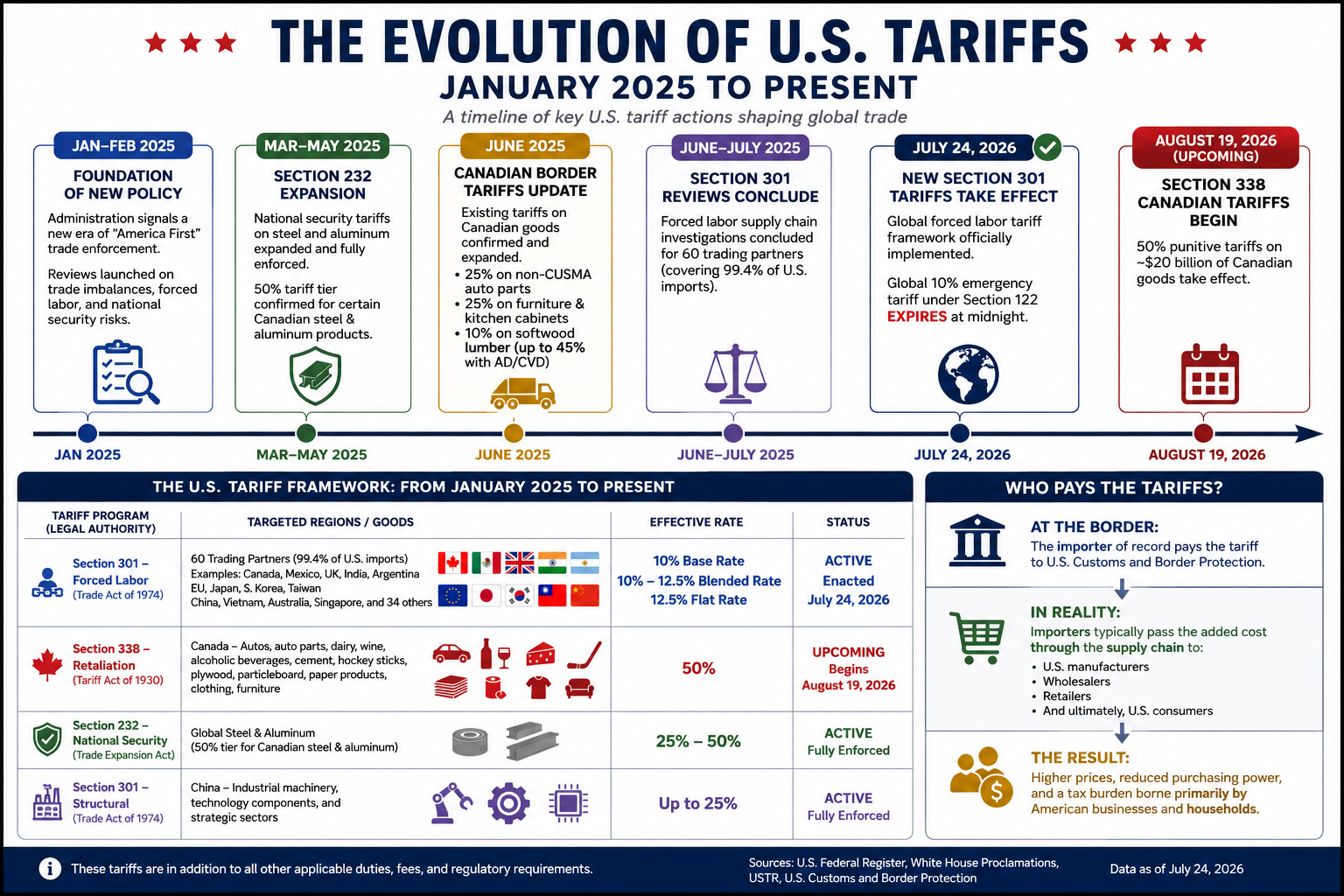
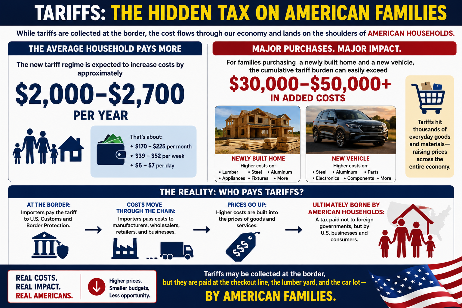
The latest U.S. tariff framework is now in place, and while tariffs are collected at the border, it’s American families who ultimately pay most of the bill.

📊 Highlights:
• Average household: +$2,000–$2,700 per year
• Buying a new home and a new car? The added cost from tariffs on steel, aluminum, lumber, vehicles, appliances, and other goods could exceed $30,000–$50,000.
• New tariffs now cover nearly 99.4% of U.S. imports from 60 trading partners, while additional 50% tariffs on many Canadian products are scheduled to begin in August.

The article explains what changed, which goods are affected, who legally pays the tariff, and who ultimately bears the economic burden.

Read the full analysis and decide for yourself: Are tariffs protecting American industry, or are they becoming one of the largest hidden taxes on American consumers?

1. Newly Enacted Tariffs: Section 301 Forced Labor Framework

Effective July 24, 2026, the United States implemented a new tariff regime targeting imports from approximately 60 trading partners, representing 99.4% of all U.S. imports. The tariffs are based on supply-chain forced labor investigations.

Tariff Rates

  • 10% Base Rate
    • Canada
    • Mexico
    • United Kingdom
    • India
    • Argentina
  • 10%–12.5% Blended Rate
    • European Union
    • Japan
    • South Korea
    • Taiwan
  • 12.5% Flat Rate
    • China
    • Vietnam
    • Australia
    • Singapore
    • 34 additional economies under investigation

Exemptions

Several strategically important commodities remain exempt, including:

  • Crude oil
  • Natural gas
  • Fertilizer
  • Selected primary food products

These tariffs also do not stack with existing Section 232 national security duties.


2. Upcoming Canadian Tariffs: Section 338

Beginning August 19, 2026, the United States is scheduled to impose 50% retaliatory tariffs on approximately $20 billion of Canadian imports under Section 338 of the Tariff Act of 1930.

Products Subject to the 50% Tariff

  • Dairy products
  • Wine and other alcoholic beverages
  • Automobiles
  • Auto parts
  • Cement
  • Hockey equipment
  • Plywood
  • Particleboard
  • Paper products
  • Clothing
  • Furniture

These tariffs bypass normal CUSMA (USMCA) preferential treatment.

Exemptions

The following Canadian exports are excluded:

  • Energy products
  • Potash
  • Fish
  • Critical minerals

3. Existing Tariffs That Remain in Effect

Several major tariff programs adopted during 2025 and 2026 continue unchanged.

Section 232 National Security Tariffs

These duties continue to apply to steel and aluminum imports, including tariffs reaching 50% on certain Canadian steel and aluminum products.

Existing Canadian Import Tariffs

Additional tariffs remain in place on:

  • 25% on non-CUSMA-compliant auto parts
  • 25% on upholstered furniture and kitchen cabinets
  • 10% tariff on Canadian softwood lumber, with combined anti-dumping and countervailing duties pushing the effective rate to approximately 45%

Section 301 China Tariffs

Long-standing tariffs on Chinese imports also remain active, with rates reaching 25% on numerous products, including:

  • Industrial machinery
  • Technology equipment
  • Electronic components
  • Strategic manufacturing inputs

Current U.S. Tariff Framework

Tariff ProgramPrimary TargetRateStatus
Section 301 – Forced Labor60 trading partners10%–12.5%Active (July 24, 2026)
Section 338 – CanadaAutos, dairy, wine, cement, consumer goods50%Begins August 19, 2026
Section 232 – National SecuritySteel & aluminum25%–50%Active
Section 301 – ChinaIndustrial & technology productsUp to 25%Active

Who Really Pays Tariffs?

Legally, tariffs are paid by the U.S. importer when goods enter the country through Customs and Border Protection.

Economically, however, that is only the beginning of the story.

Importers generally recover those additional costs by increasing the prices they charge wholesalers, retailers, manufacturers, and ultimately consumers. Numerous economic studies of recent U.S. tariffs have found that most of the cost is passed through to American businesses and households rather than absorbed by foreign exporters.

In some industries, foreign suppliers may reduce prices to remain competitive, meaning they share part of the burden. But the overall trade data and pricing evidence show that the majority of tariff costs are ultimately borne within the United States through higher prices, reduced business margins, or both.

In other words, while tariffs are collected at the border from importers, they function much like a domestic consumption tax. The final bill is usually paid by American businesses and consumers—not by foreign governments.

Conclusion

For the average American household, the new tariff regime is expected to increase costs by approximately $2,000–$2,700 per year. For families purchasing a newly built home and a new vehicle, the cumulative tariff burden can easily exceed $30,000–$50,000 through higher prices on construction materials, automobiles, appliances, and other imported goods. While tariffs are collected at the border from importers, they are ultimately borne by American businesses and consumers in the form of higher prices—a tax paid not to foreign governments, but by U.S. households.

bookmark_borderOil: A Slippery Slope (Literally and Figuratively)

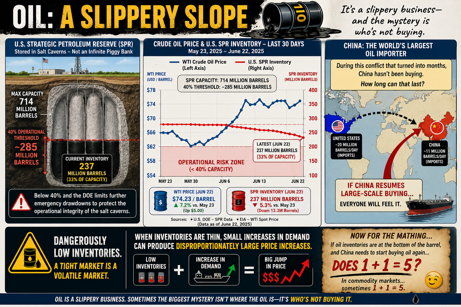
Oil is one of those subjects that’s surprisingly slippery—both physically and economically. Most people know prices go up and down, but few realize that even storing oil comes with limits.

Take the U.S. Strategic Petroleum Reserve (SPR). It’s often treated like a giant underground gas tank that can be drained and refilled at will. Not quite. The reserve is stored in massive salt caverns, and if inventories fall below roughly 40% of its 714 million-barrel capacity (about 285 million barrels), the Department of Energy limits additional emergency withdrawals. The reason isn’t politics—it’s geology. Keeping enough oil in the caverns helps maintain their long-term operational integrity.

The same basic challenge applies everywhere. Oil storage isn’t as simple as stacking barrels in a warehouse. Tanks, pipelines, and underground caverns all have practical operating limits, and those limits can shape energy policy as much as supply and demand.

Then there’s China.

Despite a conflict that many expected would trigger a buying spree, China has reportedly remained on the sidelines for months rather than aggressively increasing crude purchases. Whether that’s because of existing inventories, weak domestic demand, economic strategy, or expectations of lower future prices is open to debate.

The interesting question isn’t whether China can avoid buying oil today. It’s how long it can continue doing so.

Eventually, inventories run down, demand changes, or market conditions shift. And when one of the world’s largest oil consumers steps back into the market, everyone notices.

Oil has always been a slippery business. Sometimes the biggest mystery isn’t where the oil is—it’s who’s not buying it.

Now for the Math…

If global oil inventories are scraping the bottom of the barrel, and the world’s largest importer suddenly has to start buying again…

…does 1 + 1 = 5?

Not in arithmetic. But in commodity markets, sometimes it feels that way.

When supply is already tight, prices don’t rise in a neat, linear fashion. A relatively small increase in demand can trigger a disproportionately large jump in price as buyers compete for the same limited barrels. Traders see it coming, futures markets react, inventories shrink even faster, and a little bit of demand can snowball into a much bigger price move.

In other words, 1 + 1 doesn’t equal 5 because the math changed—it equals 5 because human behavior did.

Oil markets have always had a nonlinear streak. When inventories are comfortable, an extra million barrels a day barely makes a ripple. But when stocks are running low and spare capacity is scarce, that same million barrels can feel like throwing a match into a room full of gasoline.

That’s why economists watch inventories just as closely as production. Sometimes the most important number isn’t how much oil is being pumped—it’s how much is left in the tank.

bookmark_borderAccounting for Climate Responsibility

by Daniel Brouse

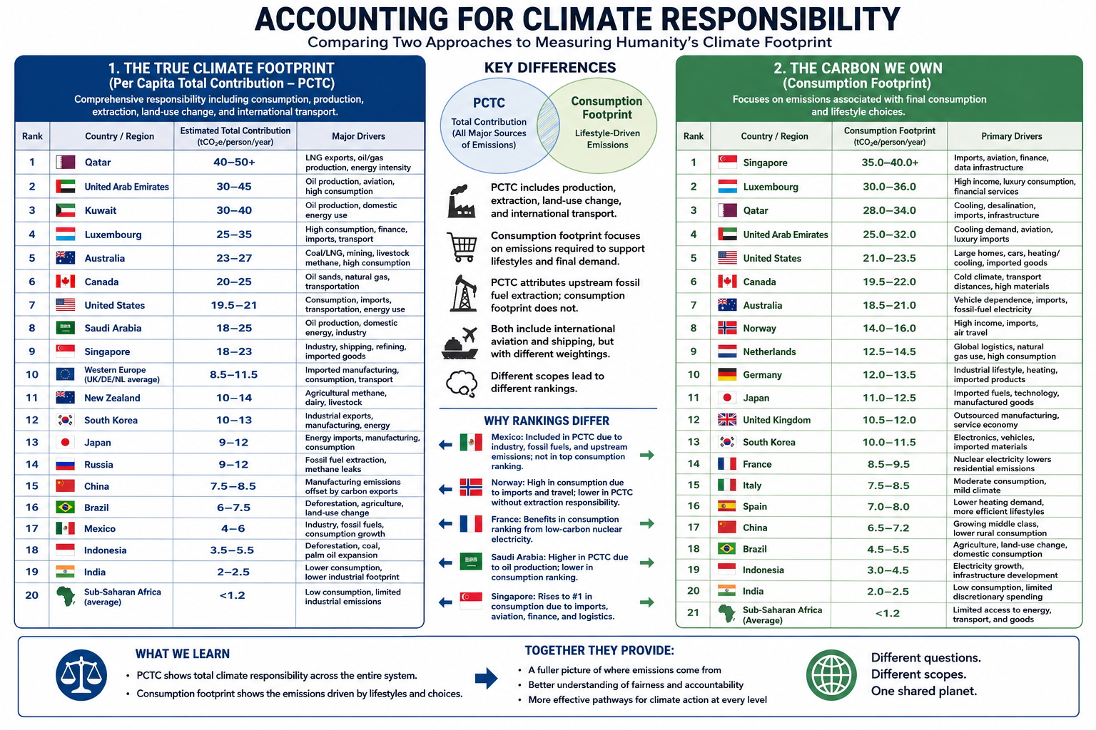
Comparing Two Approaches to Measuring Humanity’s Climate Footprint

Climate responsibility depends on how emissions are assigned. Traditional territorial accounting attributes emissions to the country where they occur, but globalization has made that approach increasingly incomplete. Modern supply chains, international trade, and service-based economies often separate where emissions are produced from who ultimately benefits from them.

To explore this problem from two different perspectives, I developed two complementary accounting frameworks.

The first paper, The True Climate Footprint: Measuring Per Capita Total Contribution Beyond Territorial Emissions, introduces the Per Capita Total Contribution (PCTC) framework. PCTC seeks to estimate an individual’s or nation’s complete climate responsibility by incorporating not only consumption, but also several major sources of emissions that are frequently omitted from conventional carbon accounting.

The True Climate Footprint: Measuring Per Capita Total Contribution

The PCTC framework includes:

  • Consumption-based emissions
  • Land-use change and deforestation
  • Upstream fossil fuel extraction (methane leakage, flaring, and coal mine emissions)
  • International aviation and maritime shipping
  • All major greenhouse gases (CO₂, CH₄, N₂O, and others expressed as CO₂-equivalent)
  • Responsibility associated with fossil fuel production where appropriate

The second paper, The Carbon We Own: Why Consumption Matters More, examines climate responsibility from a different perspective. Rather than estimating total climate contribution, it focuses specifically on the carbon footprint required to support modern lifestyles using a consumption-based accounting approach.

The Carbon We Own: Why Consumption Matters More

This framework emphasizes:

  • Multi-Regional Input-Output (MRIO) accounting
  • Direct household energy use
  • Embedded emissions in imported goods
  • Public and private services
  • Lifestyle and purchasing choices

Unlike PCTC, this framework intentionally places less emphasis on fossil fuel extraction and producer responsibility in order to better isolate the climate impacts associated with everyday consumption.

After completing the first paper, I wanted to examine the climate footprint from the perspective of the consumer rather than the entire climate system. The PCTC framework provides a comprehensive measure of total responsibility, but it does not distinguish as clearly between emissions driven by individual lifestyle choices and those associated with resource extraction or national production.

A consumption-based framework highlights decisions that individuals and societies can influence more directly. Choices such as lowering a home’s thermostat, improving insulation, selecting public transportation or electric vehicles instead of internal combustion vehicles, reducing air travel, or purchasing fewer carbon-intensive goods become more visible within the accounting. It also better captures the increasingly important role of service-based economies. While services may appear less energy-intensive than manufacturing, sectors such as healthcare, finance, telecommunications, cloud computing, and artificial intelligence rely on extensive digital infrastructure—including energy-hungry data centers—that can be substantially underrepresented in traditional emissions inventories.

Finally, I wanted a more detailed comparison among developed economies, particularly within Europe. Countries such as Norway and France illustrate why accounting methodology matters. Norway has one of the world’s cleanest domestic electricity systems, powered primarily by hydropower, yet it is also a major exporter of oil and natural gas. France, by contrast, derives much of its electricity from nuclear power, resulting in comparatively low-carbon domestic energy while maintaining a high standard of living. Comparing these countries under both frameworks reveals how different accounting methods assign responsibility and helps illustrate the strengths and limitations of each approach.

Taken together, these two papers do not compete—they answer different questions. Per Capita Total Contribution (PCTC) asks, What is humanity’s full climate responsibility? Consumption-based accounting asks, What emissions are required to sustain the lifestyle of the average resident? Used together, they provide a more complete understanding of climate responsibility than either framework alone.

Conclusion

Although The True Climate Footprint and The Carbon We Own both seek to improve upon traditional territorial emissions accounting, they answer different questions because they are built on different accounting frameworks.

The True Climate Footprint uses the Per Capita Total Contribution (PCTC) framework to estimate an individual’s or nation’s complete contribution to climate change. It extends beyond consumption to include land-use change, upstream fossil fuel extraction, international shipping and aviation, and the full spectrum of greenhouse gases. In some cases, it also attributes responsibility associated with fossil-fuel production, providing a broad measure of humanity’s total climate impact.

By contrast, The Carbon We Own focuses specifically on consumption-based climate responsibility. Using Multi-Regional Input-Output (MRIO) accounting, it assigns emissions to the final consumer by emphasizing direct household energy use, embedded emissions in imported goods, services, and lifestyle choices. It intentionally deemphasizes extraction and producer responsibility in order to better represent the carbon footprint required to sustain modern patterns of consumption.

Because these frameworks measure different aspects of climate responsibility, their rankings are not expected to be identical.

Mexico provides a useful illustration. Under the PCTC framework, Mexico’s estimated footprint includes domestic industry, fossil fuel production, growing consumption, and upstream emissions, resulting in an estimated contribution of approximately 4–6 tonnes of CO₂-equivalent per person per year. In the consumption-based analysis, however, Mexico does not appear among the highest-ranking countries because the focus is limited to end-user consumption, and the published rankings emphasize the world’s largest per-capita consumption footprints.

Similar differences appear elsewhere. Norway’s position changes substantially because one framework incorporates the climate responsibility associated with fossil fuel production, while the other emphasizes domestic consumption. France benefits in the consumption-based analysis because its low-carbon nuclear electricity reduces household emissions despite maintaining a high standard of living. Saudi Arabia ranks differently depending on whether responsibility is assigned to oil production or to energy consumption. Singapore rises dramatically under consumption accounting because imported goods, international aviation, finance, logistics, and digital infrastructure contribute heavily to its consumption footprint despite relatively limited domestic manufacturing.

These examples demonstrate that accounting methodology influences how climate responsibility is distributed. Production-based, consumption-based, and total-contribution frameworks each illuminate different dimensions of the global climate system.

Rather than viewing these approaches as competing methodologies, they should be regarded as complementary analytical tools. The Per Capita Total Contribution (PCTC) framework asks, What is a nation’s or individual’s total contribution to climate change? The consumption-based framework asks, What emissions are required to sustain the average resident’s lifestyle? Together, they provide a more complete understanding of climate responsibility than either approach can achieve alone, revealing both the systemic impacts of resource production and the powerful role of consumer demand in shaping the global climate.

bookmark_borderThe Carbon We Own: Why Consumption Matters More

by Daniel Brouse

For decades, climate responsibility has often been measured by where fossil fuels are extracted or where products are manufactured. While useful for tracking national emissions, this production-based approach can misrepresent who ultimately drives demand.

A consumption-based accounting approach shifts the focus to the end user. Instead of assigning emissions to the country where a product is made, it attributes emissions to the people and businesses that ultimately consume the energy, goods, and services.

Under this framework, every kilowatt-hour of electricity, every heating bill, every medical service, and every consumer product is assigned to its final destination.

For example, if a smartphone is manufactured in Asia using electricity generated from coal and then shipped across the Pacific to a consumer in Los Angeles, the emissions associated with mining, manufacturing, transportation, and delivery are attributed to the American consumer—not the manufacturing country.

This approach provides a more accurate picture of the carbon footprint associated with modern lifestyles.


How Consumption-Based Carbon Accounting Works

Most consumption analyses rely on Multi-Regional Input-Output (MRIO) economic models, which trace emissions through global supply chains before assigning them to final consumers.

Individual carbon footprints are generally divided into three major categories:

1. Direct Household Energy

Emissions from energy used directly by households, including:

  • Home heating and cooling
  • Residential electricity
  • Personal vehicle fuel
  • Digital activities such as internet usage and streaming services

2. Embedded Goods

Emissions generated while producing and transporting purchased products, including:

  • Electronics
  • Vehicles
  • Furniture
  • Clothing
  • Building materials
  • Household appliances

These emissions often occur in countries far from the final consumer.

3. Services

Many of the largest emissions in developed economies come not from physical products but from services, including:

  • Healthcare
  • Commercial aviation
  • Banking and finance
  • Cloud computing
  • Water and wastewater treatment
  • Telecommunications

In the United States alone, healthcare contributes roughly 1.6 tonnes of CO₂-equivalent emissions per person each year, illustrating how service-based economies can generate substantial carbon footprints even as heavy industry declines.


Major Findings from Global Consumption Accounting

The Rise of Service Economies

In wealthy economies such as Singapore, Luxembourg, and several Western European countries, manufacturing represents only a small portion of domestic emissions.

Instead, much of their climate impact comes from:

  • Commercial aviation
  • Financial systems
  • Cloud computing
  • Global logistics
  • Luxury consumption
  • High levels of imported goods

As economies become increasingly service-oriented, carbon emissions become embedded in complex international supply chains rather than local smokestacks.


Geography Still Matters

Climate strongly influences direct household energy use.

Countries with long, cold winters or extremely hot summers require substantially more energy for climate control.

For example:

  • Canada and the United States consume large amounts of energy for winter heating and summer air conditioning, particularly because of larger average home sizes.
  • Australia records comparatively higher emissions from agriculture, mining, and infrastructure development than from residential heating.

Local climate remains an important contributor even after imported goods are included.


China’s Manufacturing Versus Consumption

China illustrates one of the largest differences between production-based and consumption-based accounting.

Because China manufactures enormous quantities of products for export, its territorial emissions are among the highest in the world.

However, when emissions are allocated to the people who ultimately purchase those products, China’s domestic per-capita consumption footprint is estimated at roughly 6.8 tonnes of CO₂-equivalent per year.

This highlights the distinction between:

  • Production emissions (where goods are made)
  • Consumption emissions (who ultimately benefits from those goods)

Many products manufactured in China are consumed in North America and Europe, meaning a significant share of manufacturing emissions is driven by foreign demand.


Consumption Footprints Across Europe

Norway: Clean Electricity, High Consumption

Estimated consumption footprint: 14.8 tonnes CO₂e per person

Norway’s electricity is more than 85% hydropower, giving it one of the cleanest electrical grids in the world.

Yet Norwegians have high purchasing power and consume large quantities of imported goods, including:

  • Electric vehicles
  • Consumer electronics
  • Luxury goods
  • Imported foods

Norway also has one of the world’s highest rates of air travel per capita, increasing its service-sector emissions.

The result is a consumption footprint considerably larger than its territorial emissions suggest.


United Kingdom: Outsourcing Manufacturing

Estimated consumption footprint: 11.2 tonnes CO₂e per person

The United Kingdom has significantly reduced domestic production emissions by retiring coal-fired power plants and expanding renewable electricity.

However, much of the country’s manufacturing has shifted overseas.

The UK imports large quantities of:

  • Electronics
  • Machinery
  • Clothing
  • Construction materials

Consequently, much of its carbon footprint exists outside its borders, while domestic emissions increasingly come from finance, digital infrastructure, commercial services, and transportation.


France: The Nuclear Advantage

Estimated consumption footprint: 9.2 tonnes CO₂e per person

France demonstrates how a low-carbon electricity system can substantially reduce consumption emissions.

French households enjoy living standards comparable to neighboring Western European countries, yet much of their residential electricity, rail transportation, and heating is supplied by nuclear energy.

As a result, France’s direct household energy emissions are estimated to be roughly 30% lower than those of many neighboring countries with similar consumption patterns.


China Compared with Western Europe

When emissions are assigned to consumers rather than producers, an average citizen in countries such as Germany or the United Kingdom is responsible for nearly twice the carbon footprint of the average Chinese citizen.

Although China’s middle class continues to grow and domestic consumption is increasing, much of the country’s industrial output still serves international markets.

This comparison illustrates a key insight of consumption-based accounting:

A nation’s production does not necessarily reflect the climate impact of its residents’ lifestyles.


A Different Way to Think About Climate Responsibility

Consumption-based accounting reframes climate responsibility by asking a simple question:

Who ultimately benefits from the energy and resources consumed?

Rather than focusing solely on where emissions occur, this approach follows products and services through global supply chains to their final users.

For affluent economies that import large volumes of manufactured goods while exporting much of their industrial production, consumption-based accounting often reveals substantially higher per-capita climate footprints than traditional territorial inventories.

Viewed through this lens, lifestyle choices, purchasing power, housing, transportation, travel, healthcare, digital services, and overall consumption patterns become the primary drivers of individual climate responsibility.

Ultimately, the atmosphere responds to total emissions, regardless of where they occur. Consumption-based accounting provides a complementary perspective to traditional production-based inventories by connecting those emissions to the people and economies whose demand created them.

Global Consumption Footprint Rankings

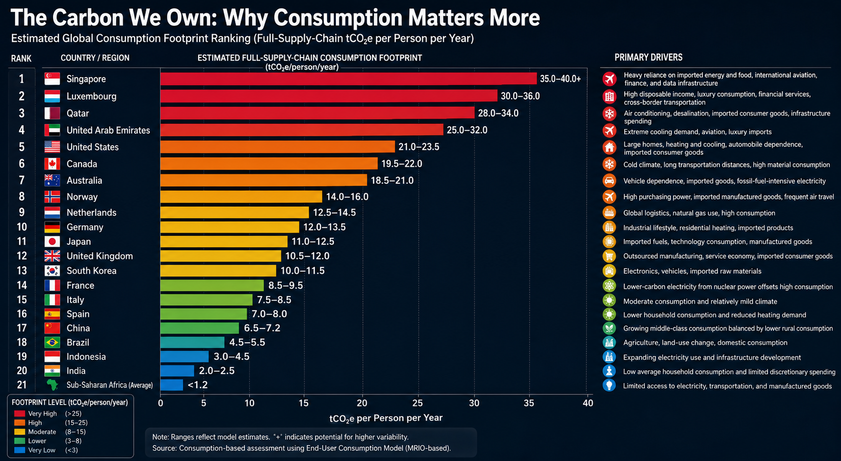
Traditional emissions inventories assign carbon pollution to the country where fossil fuels are extracted or products are manufactured. A consumption-based accounting approach instead assigns those emissions to the people and economies that ultimately consume the goods and services.

The rankings below are based on an End-User Consumption Model, which allocates the full upstream supply-chain emissions—including raw material extraction, manufacturing, international transportation, agricultural land-use change, and other embedded emissions—to the final purchaser.

Rather than measuring where emissions occur, this framework estimates the carbon footprint required to sustain the average lifestyle of a country’s residents. It reflects direct household energy use, consumption of imported goods, transportation, public infrastructure, and carbon-intensive services.

Estimated Global Consumption Footprint Ranking

RankCountry / RegionEstimated Full-Supply-Chain Consumption Footprint (tCO₂e/person/year)Primary Drivers
1🇸🇬 Singapore35.0–40.0+Heavy reliance on imported energy and food, international aviation, finance, and data infrastructure
2🇱🇺 Luxembourg30.0–36.0High disposable income, luxury consumption, financial services, cross-border transportation
3🇶🇦 Qatar28.0–34.0Air conditioning, desalination, imported consumer goods, infrastructure spending
4🇦🇪 United Arab Emirates25.0–32.0Extreme cooling demand, aviation, luxury imports
5🇺🇸 United States21.0–23.5Large homes, heating and cooling, automobile dependence, imported consumer goods
6🇨🇦 Canada19.5–22.0Cold climate, long transportation distances, high material consumption
7🇦🇺 Australia18.5–21.0Vehicle dependence, imported goods, fossil-fuel-intensive electricity
8🇳🇴 Norway14.0–16.0High purchasing power, imported manufactured goods, frequent air travel
9🇳🇱 Netherlands12.5–14.5Global logistics, natural gas use, high consumption
10🇩🇪 Germany12.0–13.5Industrial lifestyle, residential heating, imported products
11🇯🇵 Japan11.0–12.5Imported fuels, technology consumption, manufactured goods
12🇬🇧 United Kingdom10.5–12.0Outsourced manufacturing, service economy, imported consumer goods
13🇰🇷 South Korea10.0–11.5Electronics, vehicles, imported raw materials
14🇫🇷 France8.5–9.5Lower-carbon electricity from nuclear power offsets high consumption
15🇮🇹 Italy7.5–8.5Moderate consumption and relatively mild climate
16🇪🇸 Spain7.0–8.0Lower household consumption and reduced heating demand
17🇨🇳 China6.5–7.2Growing middle-class consumption balanced by lower rural consumption
18🇧🇷 Brazil4.5–5.5Agriculture, land-use change, domestic consumption
19🇮🇩 Indonesia3.0–4.5Expanding electricity use and infrastructure development
20🇮🇳 India2.0–2.5Low average household consumption and limited discretionary spending
21Sub-Saharan Africa (Average)<1.2Limited access to electricity, transportation, and manufactured goods

Key Patterns

Small, Wealthy Nations Have the Largest Per-Capita Footprints

Singapore and Luxembourg rank highest despite having relatively little domestic heavy industry. Their residents consume large quantities of imported goods and services, while extensive international transportation, finance, aviation, and digital infrastructure contribute substantial embedded emissions.

High-Income, Car-Oriented Economies Form the Next Tier

The United States, Canada, and Australia consistently rank among the world’s largest per-capita consumers. Large homes, automobile-dependent communities, extensive heating or cooling needs, and high levels of discretionary consumption combine to produce substantial lifestyle-related emissions.

Low-Carbon Electricity Helps—but Doesn’t Eliminate Consumption Emissions

Countries such as France and Norway demonstrate that cleaner electricity significantly lowers household energy emissions. However, imported goods, international travel, and service-sector activities remain important contributors to their overall consumption footprints.

Manufacturing Countries Are Not Necessarily the Largest Consumers

China’s production-based emissions are among the highest globally because it manufactures goods for international markets. Under a consumption-based framework, however, the average Chinese citizen’s lifestyle footprint remains considerably lower than that of residents in many affluent Western countries.

Consumption Capacity Is the Strongest Predictor

Perhaps the clearest finding is the enormous gap between affluent economies and developing regions. Average per-capita consumption in Sub-Saharan Africa remains a small fraction of that in the world’s wealthiest nations, reflecting differences in income, energy access, transportation, housing, and consumer purchasing power.

This comparison underscores a central conclusion of consumption-based accounting: the carbon footprint of an individual is driven primarily by the scale and complexity of the lifestyle they support, rather than the geographic location where the associated emissions physically occur.

bookmark_borderThe True Climate Footprint: Measuring Per Capita Total Contribution

by Daniel Brouse

Why Traditional Carbon Accounting Underestimates Responsibility

Climate responsibility is often measured using territorial emissions: the greenhouse gases released within a country’s borders. While useful, this approach does not capture the full climate footprint of modern economies because it ignores global supply chains, outsourced manufacturing, land-use change, and upstream fossil fuel emissions.

A more complete measure requires calculating Per Capita Total Contribution—a footprint-based accounting system that assigns responsibility based on the full lifecycle of consumption and environmental impact.

This approach combines:

  • Consumption-based emissions accounting — tracking emissions embedded in imported goods and services.
  • Land Use Change (LUC) — including deforestation, agricultural expansion, and ecosystem conversion.
  • Upstream fossil fuel emissions — including methane leaks, flaring, and coal mine emissions.
  • International transportation — including aviation and shipping.
  • All greenhouse gases — not just carbon dioxide, but methane, nitrous oxide, and other climate pollutants.

Using this broader framework, humanity’s total annual climate footprint rises to approximately 53.5 billion tonnes of CO₂-equivalent (CO₂e), or about 6.6 tonnes of CO₂e per person globally.

However, once these factors are included, the global map of climate responsibility changes dramatically.


1. The Hidden Carbon Footprint of Global Trade

Outsourced Emissions: When Consumption Drives Pollution Elsewhere

Traditional accounting assigns emissions to the country where goods are produced. This creates a major distortion in a globalized economy.

Consumption-based accounting reverses this by:

  • Subtracting emissions from exports.
  • Adding emissions embedded in imports.
  • Assigning responsibility to the final consumer.

This reveals a significant shift:

Western Consumption Footprints Expand

Many wealthy nations have reduced domestic industrial emissions partly by moving manufacturing overseas. Electronics, clothing, machinery, and other consumer products may be manufactured in China or Southeast Asia, but much of the demand originates in North America and Europe.

The emissions occur in the producing country, but the consumption benefit occurs elsewhere.

Carbon Exporters vs. Carbon Importers

Under territorial accounting:

  • Manufacturing nations appear more responsible.
  • Consumer nations appear cleaner.

Under footprint accounting:

  • Major consumer economies become large net importers of carbon emissions.
  • Manufacturing hubs become net exporters of embedded carbon.

2. The Missing Climate Cost of Land Use Change

Deforestation and land conversion contribute roughly 10% of global greenhouse gas emissions.

However, these emissions are rarely assigned to the ultimate consumers driving demand.

A complete accounting system tracks:

  • Beef production linked to Amazon clearing.
  • Soy expansion replacing forests.
  • Palm oil plantations.
  • Timber extraction.
  • Agricultural conversion.

Consumer-Driven Deforestation Footprints

Some nations experience a substantial increase in their climate footprint when imported commodities are included.

Examples:

  • Wealthy food-importing nations may carry a larger footprint because their consumption drives land clearing elsewhere.
  • Countries such as Brazil and Indonesia receive major additions from domestic land-use change before those emissions are redistributed through trade.

3. Fossil Fuel Extraction: Counting the Full Climate Cost

Burning fossil fuels is only part of their climate impact.

A complete footprint must include emissions from extraction:

  • Methane leakage from oil and gas production.
  • Coal mine methane releases.
  • Flaring.
  • Venting during production and transport.

Methane is especially important because it is approximately 30 times more powerful than carbon dioxide over a 100-year period.

Territorial accounting can distort responsibility:

  • Fossil fuel exporters may appear responsible for extraction emissions occurring within their borders.
  • Consumer nations benefit from the energy but avoid the associated extraction footprint.

A true accounting system assigns these emissions across the entire fossil fuel supply chain, including the countries ultimately consuming the energy.


The Recalculated Climate Responsibility Landscape

Country / RegionStandard Territorial CO₂ (Fossil Fuels Only)Estimated Total Contribution (All GHGs + Trade + Land Use + Transport)Primary Driver of Change
United States~14.9 tonnes/person~19.5–21.0 tonnes/personHigh consumption, imported manufacturing, carbon-intensive lifestyles
Western Europe~4.5–7.0 tonnes/person~8.5–11.5 tonnes/personOutsourced manufacturing and imported goods
China~8.0 tonnes/person~7.5–8.5 tonnes/personLarge manufacturing exporter offsets domestic emissions
Brazil~2.3 tonnes/person~6.0–7.5 tonnes/personDeforestation and agricultural land conversion
India~2.0 tonnes/person~2.2 tonnes/personLower consumption footprint
Sub-Saharan Africa<1.0 tonnes/person<1.2 tonnes/personLow consumption and limited industrial emissions

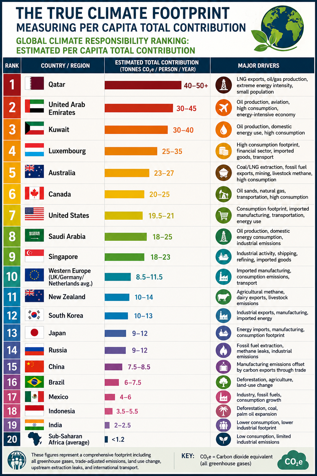
Global Climate Responsibility Ranking: Estimated Per Capita Total Contribution

RankCountry / RegionEstimated Total Contribution (Tonnes CO₂e/person/year)Major Drivers
1Qatar40–50+LNG exports, oil/gas production, extreme energy intensity, small population
2United Arab Emirates30–45Oil production, aviation, high consumption, energy-intensive economy
3Kuwait30–40Oil production, domestic energy use, high consumption
4Luxembourg25–35High consumption footprint, financial sector, imported goods, transport
5Australia23–27Coal/LNG extraction, fossil fuel exports, mining, livestock methane, high consumption
6Canada20–25Oil sands, natural gas, transportation, high consumption
7United States19.5–21Consumption footprint, imported manufacturing, transportation, energy use
8Saudi Arabia18–25Oil production, domestic energy consumption, industrial emissions
9Singapore18–23Industrial activity, shipping, refining, imported goods
10Western Europe (UK/Germany/Netherlands average)8.5–11.5Imported manufacturing, consumption emissions, transport
11New Zealand10–14Agricultural methane, dairy exports, livestock emissions
12South Korea10–13Industrial exports, manufacturing, imported energy
13Japan9–12Energy imports, manufacturing, consumption footprint
14Russia9–12Fossil fuel extraction, methane leaks, industrial emissions
15China7.5–8.5Manufacturing emissions offset by carbon exports through trade
16Brazil6–7.5Deforestation, agriculture, land-use change
17Mexico4–6Industry, fossil fuels, consumption growth
18Indonesia3.5–5.5Deforestation, coal, palm oil expansion
19India2–2.5Lower consumption, lower industrial footprint
20Sub-Saharan Africa (average)<1.2Low consumption, limited industrial emissions

The Real Climate Equation: Consumption × Population × Technology

The climate challenge is often framed as a population problem. However, the dominant driver of emissions is not simply the number of people on Earth—it is the per capita intensity of resource consumption and pollution.

A more accurate equation is:Total Climate Impact=Population×Per Capita Consumption×Carbon Intensity\textbf{Total Climate Impact} = \textbf{Population} \times \textbf{Per Capita Consumption} \times \textbf{Carbon Intensity}Total Climate Impact=Population×Per Capita Consumption×Carbon Intensity

Population matters, but consumption patterns and technology determine the magnitude of environmental impact.

A world with billions more people using efficient, low-carbon systems could have a smaller footprint than a smaller population consuming resources at current high-intensity levels.


Toward a Fairer Climate Accounting System

Territorial emissions remain useful for tracking national inventories, but they do not fully capture responsibility in a globalized economy.

A true Per Capita Total Contribution framework recognizes that climate change is driven by:

  • Who consumes resources.
  • Who benefits from production.
  • Who drives land conversion.
  • Who extracts and burns fossil fuels.
  • Who has the technological and economic capacity to reduce emissions.

The future of climate accountability depends on moving beyond borders and measuring the complete human footprint on Earth.


Conclusion

The climate conversation has focused on the wrong number.

The problem isn’t simply how many people live on Earth.

It’s how each of us lives.

The average person on the planet is responsible for about 6.6 tonnes of CO₂e per year, but the differences between countries are staggering. Some affluent societies generate 20–50+ tonnes per person, while much of the developing world contributes less than 2 tonnes.

That’s why climate responsibility is better measured by per capita total contribution—including consumption, outsourced manufacturing, deforestation, fossil fuel extraction, agriculture, and transportation—not just emissions produced within national borders.

A child born into a high-consumption lifestyle can have a climate footprint many times larger than several people living in low-consumption economies.

The challenge is not humanity itself.

The challenge is how we consume, how we produce, and how much we extract from the planet.

Changing lifestyles, improving efficiency, and transitioning to cleaner energy can reduce our impact without reducing our humanity.

The future depends less on the number of people—and more on the choices each of us makes.


bookmark_borderWhat Are the Odds? An Estate Plan for the Next Seven Generations

by Daniel Brouse and Sidd Mukherjee

When I began this journey more than three decades ago, I wasn’t a climate researcher. I was a financial planner specializing in business, economics, estate planning, and risk management. My academic background included economics, philosophy, and extensive study in physics, calculus, statistics, and systems analysis. My career focused on a simple question:

How do you create the best possible future for the people who come after you?

In the early 1990s, I met a brilliant scientist named Sidd. We shared a curiosity about complex systems and a desire to test ideas rather than simply debate them. Together, we began an experiment that has now spanned more than thirty years.

Our goal was unusual. We wanted to build what we jokingly called a one-size-fits-all, bulletproof shareware estate plan—not for one family, but for every family on Earth.

At the same time, I was helping pioneer some of the earliest privately owned web servers. Before commercial hosting became commonplace, we were operating online while many organizations were still connected through universities. It was the same era when Yahoo! itself was running from Stanford University.

By 1995, our website, KingArthur.com, was attracting millions of visitors each month. The internet gave us something few researchers had ever possessed: the ability to interact directly with millions of people across cultures, countries, religions, and generations.

One question became central to our experiment:

“When it comes to your life and what you leave behind, what is the single most important thing?”

We expected many people to answer with wealth, success, fame, or legacy.

Instead, they overwhelmingly answered something much simpler.

Among people under fifty, the most common answer was their children.

Among those over fifty, the answer shifted to their grandchildren.

The experiment revealed something profound. The greatest wealth most people hope to preserve is not money. It is the opportunity for future generations to experience the same joys they have experienced themselves.

In other words, the ultimate estate plan is remarkably simple:

To my children’s children’s children.

The greatest inheritance most of us hope to leave is not a larger bank account. It is the chance for our descendants to raise children of their own, watch them grow, and someday become grandparents themselves.

When we began this experiment, I did not have grandchildren.

Today I do.

That changes everything.

Coincidentally, I was recently asked a question that perfectly captured the purpose of this work:

“Can you play with me on this? I’m wearing my nutritional ecologist hat here, and I’m in a municipal-level discussion that is trying to zoom out seven generations while also identifying the baby steps needed over the next four-year election cycle.”

My immediate thought was:

Exactly.

That is what this experiment has always been about.

An estate plan should not end with our children—or even our grandchildren. It should extend seven generations into the future.

My grandchildren deserve the opportunity to become grandparents themselves. Their grandchildren deserve the same opportunity.

That is entirely achievable—but only if we make wise decisions today.

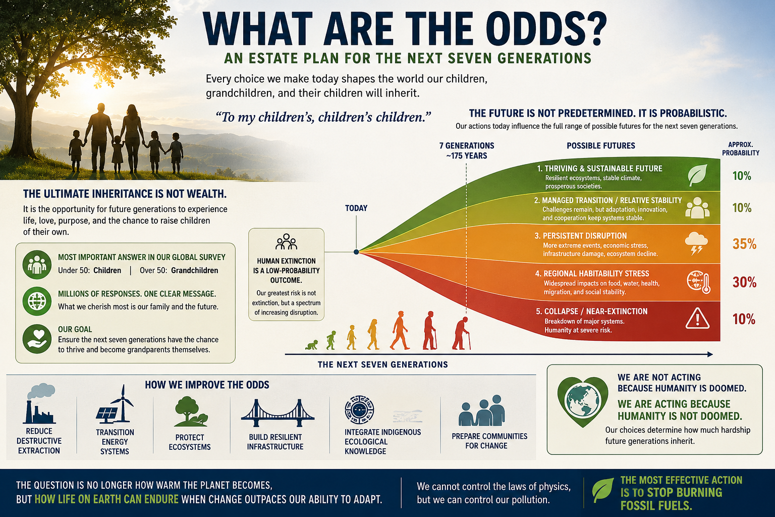
The graph that follows illustrates that idea.

Every choice we make now influences the range of possible futures available to the next seven generations.

Some outcomes are relatively optimistic. Some involve increasing climate disruption.

Some are far more severe.

Importantly, human extinction remains a low-probability outcome.

The far more likely future is not one of sudden extinction, but one that spans a spectrum of increasing disruption—affecting ecosystems, agriculture, infrastructure, economies, public health, migration, and regional habitability.

The probabilities are not fixed. They are shaped by the decisions humanity makes over the coming decades.. including today.

That changes the conversation entirely.

The question is no longer:

“Are humans going extinct?”

The more important question is:

“How difficult do we want life to be for the next seven generations?”

That question naturally leads to practical priorities:

  • Reduce destructive extraction of fossil fuels and natural resources.
  • Transition to cleaner and more resilient energy systems.
  • Protect and restore forests, wetlands, and other ecosystems.
  • Build infrastructure capable of withstanding future climate conditions.
  • Integrate Indigenous ecological knowledge alongside modern science.
  • Prepare communities to adapt to unavoidable change.

The most important message is this:

We are not acting because humanity is doomed.

We are acting because humanity is not doomed.

Our choices today determine how much hardship future generations inherit.

Ultimately, this is not simply a discussion about climate change.

It is an estate planning exercise on a planetary scale.

The question is no longer how warm the planet becomes.

The question is how well civilization—and the generations that follow us—can endure as environmental change accelerates faster than our ability to adapt.

We cannot rewrite the laws of physics. But we can decide how much pollution we continue to add to the atmosphere.

The most effective step we can take is also the simplest:

Stop burning fossil fuels as quickly and responsibly as possible, while building a more resilient world for the generations that follow.

bookmark_borderClimate Change: A Theoretical 200-Year Probability Envelope

by Daniel Brouse

Derived from the Nonlinear Acceleration Framework

Model Time Horizon:

2026–2226

Outcome Categories:

  1. Climate Stabilization / Managed Transition
  2. Increasing Climate Disruption
  3. Regional Habitability Stress
  4. Global System Stress
  5. Civilization-Scale Contraction
  6. Human Extinction Boundary

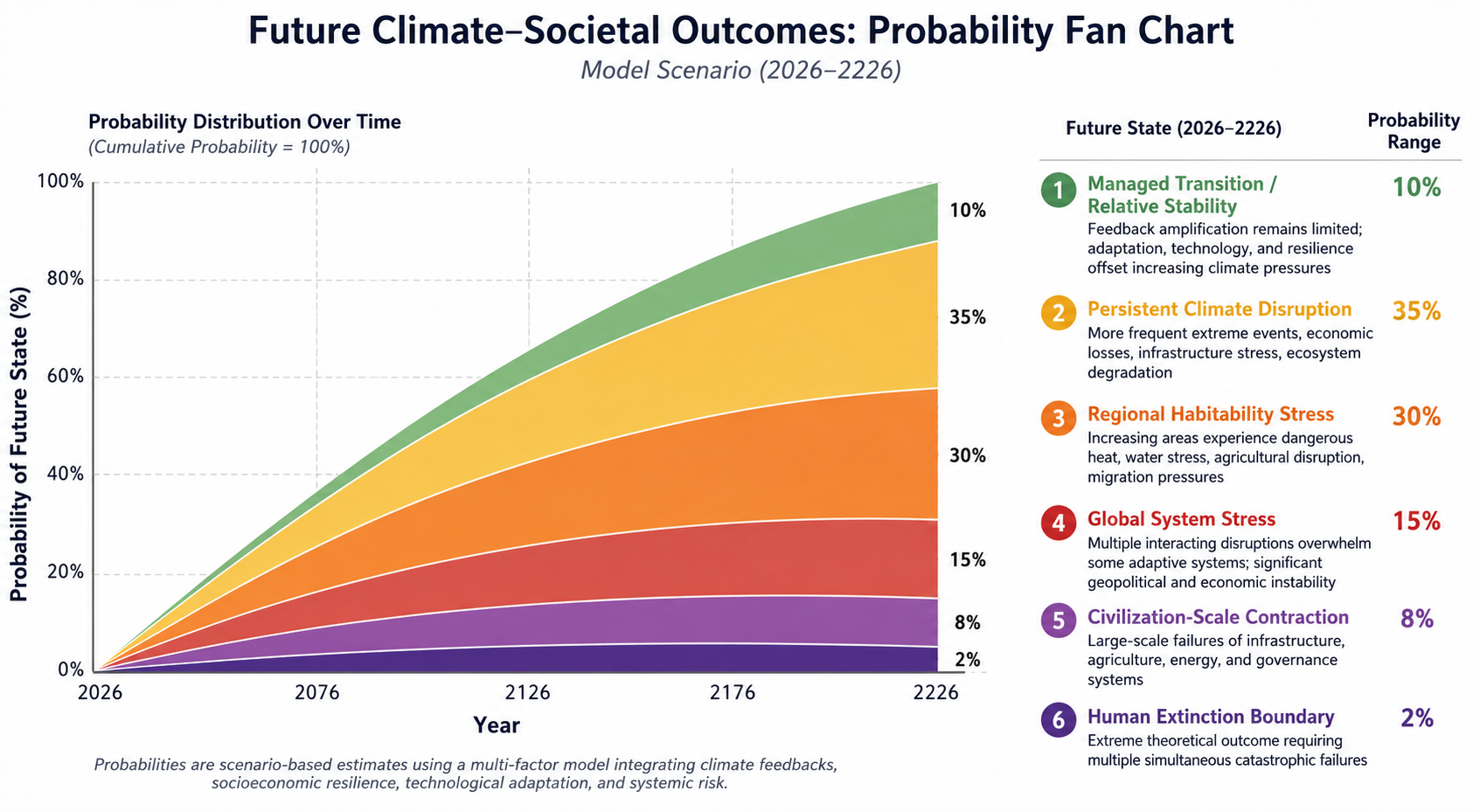
Probability Distribution (Model Scenario)

Future State (2026–2226)Probability RangeFramework Interpretation
1. Managed Transition / Relative Stability10%Feedback amplification remains limited; adaptation, technology, and resilience offset increasing climate pressures
2. Persistent Climate Disruption35%More frequent extreme events, economic losses, infrastructure stress, ecosystem degradation
3. Regional Habitability Stress30%Increasing areas experience dangerous heat, water stress, agricultural disruption, migration pressures
4. Global System Stress15%Multiple interacting disruptions overwhelm some adaptive systems; significant geopolitical and economic instability
5. Civilization-Scale Contraction8%Large-scale failures of infrastructure, agriculture, energy, and governance systems
6. Human Extinction Boundary2%Extreme theoretical outcome requiring multiple simultaneous catastrophic failures

Probability Envelope Visualization

Probability of Future States (2026–2226)

Managed Transition
██████████ 10%

Persistent Disruption
███████████████████████████████████ 35%

Regional Habitability Stress
██████████████████████████████ 30%

Global System Stress
███████████████ 15%

Civilization Contraction
████████ 8%

Human Extinction Boundary
██ 2%

How the Distribution Changes Over Time

The framework assumes that probability is not static.

The distribution evolves as system coupling changes.


Period 1: 2026–2050

Early Acceleration Phase

Dominant processes:

Climate Stress → Extreme Events → Infrastructure Costs → Adaptation Pressure

Estimated distribution:

OutcomeProbability
Managed transition20%
Persistent disruption50%
Regional stress25%
Global stress5%
Civilization contraction<1%
Extinction boundary<1%

Interpretation:

The system remains largely within existing civilization structures, but disruption increases.


Period 2: 2050–2100

Coupling Expansion Phase

Dominant processes:

Multiple Feedbacks → Compound Events → Reduced Recovery Time → Greater System Sensitivity

Estimated distribution:

OutcomeProbability
Managed transition10%
Persistent disruption40%
Regional stress35%
Global stress12%
Civilization contraction3%
Extinction boundary<1%

Interpretation:

The primary shift is from isolated events toward interacting disruptions.


Period 3: 2100–2200

System Transition Phase

Dominant processes:

Climate Stress × Ecosystem Stress × Infrastructure Stress

Estimated distribution:

OutcomeProbability
Managed transition5%
Persistent disruption25%
Regional stress35%
Global stress25%
Civilization contraction9%
Extinction boundary1%

Interpretation:

The probability envelope broadens because uncertainty increases as multiple systems interact.


Period 4: 2200–2226

Long-Term Equilibrium Selection

Possible pathways:

Pathway A: Adapted Earth System

Stress<ResilienceStress < Resilience

Outcome:

Stable but transformed civilization


Pathway B: High-Stress Earth System

Stress≈ResilienceStress \approx Resilience

Outcome:

Persistent disruption and regional instability


Pathway C: Cascading Failure

Stress>ResilienceStress > Resilience

Outcome:

Civilization contraction


The Framework’s Core Equation

A simplified representation:Future Risk=Climate Stress×Feedback Coupling×Acceleration×VulnerabilityResilienceFuture\ Risk = \frac{ Climate\ Stress \times Feedback\ Coupling \times Acceleration \times Vulnerability } { Resilience }


Interpretation of the Upper Boundary

The framework separates:

Planetary Habitability

from:

Human Civilization

The probability hierarchy is:P(Climate Disruption)>P(Regional Stress)>P(Civilization Collapse)>P(Human Extinction)P(Climate\ Disruption) > P(Regional\ Stress) > P(Civilization\ Collapse) > P(Human\ Extinction)

The model therefore treats human extinction as a low-probability upper boundary, not the central pathway.

The more probable outcome under increasing nonlinear acceleration is:

A progressively more difficult Earth for existing human systems to operate within.


Sensitivity Analysis

The largest factors shifting the probability envelope would be:

VariableEffect
Feedback coupling increasesMoves probability toward disruption
Acceleration increasesCompresses response time
Ecosystem degradation increasesRaises vulnerability
Adaptation improvesMoves probability toward stability
Resilience declinesRaises systemic risk
Feedbacks weakenMoves probability toward stabilization

Summary Distribution

The theoretical 200-year envelope:

Most Probable Region:

Persistent Disruption
        ↓
Regional Habitability Stress


Less Probable:

Global System Stress
        ↓
Civilization Contraction


Extreme Upper Boundary:

Human Extinction

Framework Conclusion

Under the Nonlinear Acceleration Framework, the primary risk is not a sudden transition from a habitable Earth to an uninhabitable planet.

The dominant theoretical risk pathway is:

Increasing Feedback Coupling → Accelerating Impacts → Reduced Recovery Time → Growing System Stress → Progressive Civilization Challenges

The extinction boundary exists as the extreme edge of the probability envelope, while the central concern is the increasing probability of a world where human systems must operate under rapidly changing environmental conditions.

bookmark_borderThe Collapse of Climate Predictability

by Daniel Brouse

How Coupled Climate Feedbacks Are Changing Earth’s Behavior

Abstract

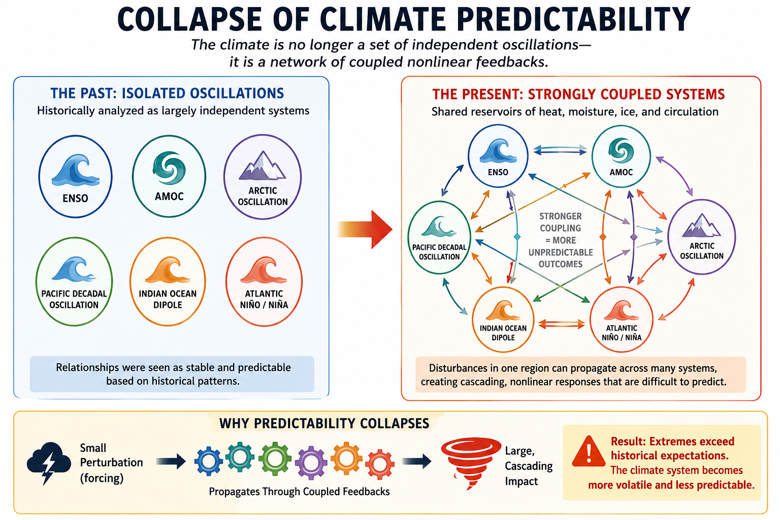
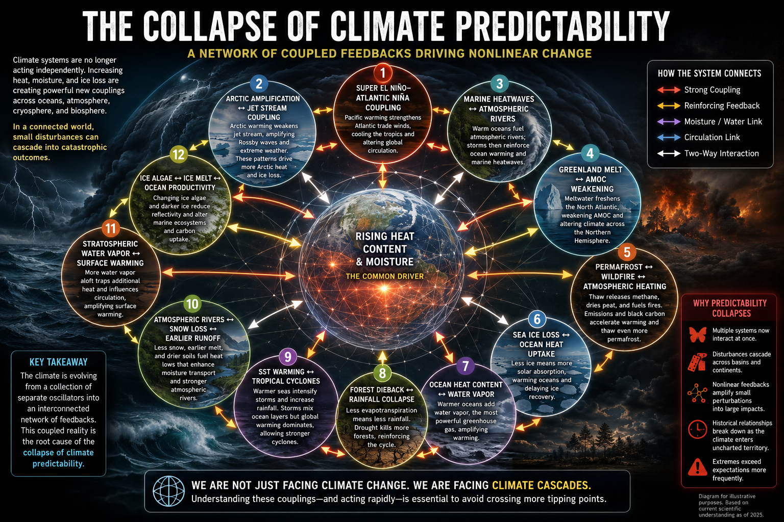
For much of the modern scientific era, Earth’s major climate oscillations were studied as largely independent systems. Phenomena such as the El Niño–Southern Oscillation (ENSO), the Atlantic Meridional Overturning Circulation (AMOC), the Arctic Oscillation (AO), the Pacific Decadal Oscillation (PDO), the Indian Ocean Dipole (IOD), and the Atlantic Niño/Niña each possessed recognizable patterns, historical relationships, and reasonably predictable behavior.

Today, however, a growing body of observations suggests these systems are becoming increasingly interconnected through shared reservoirs of heat, moisture, ice, and atmospheric circulation. Rather than behaving as isolated oscillators, they are evolving into a tightly coupled network in which disturbances propagate across multiple components of the Earth system. This increasing connectivity reduces the reliability of historical climate relationships and contributes to what can be described as the collapse of climate predictability.


From Independent Oscillators to a Coupled System

Classical climatology often treated Earth’s major modes of variability as separate oscillations whose interactions were relatively weak and occurred over well-defined time scales.

Examples include:

  • El Niño–Southern Oscillation (ENSO)
  • Atlantic Meridional Overturning Circulation (AMOC)
  • Arctic Oscillation (AO)
  • Pacific Decadal Oscillation (PDO)
  • Indian Ocean Dipole (IOD)
  • Atlantic Niño/Niña

These oscillations remain useful conceptual tools, but they no longer appear to behave as isolated components. Instead, they increasingly exchange energy through atmospheric circulation, ocean heat transport, cryospheric change, and hydrologic feedbacks.

The climate system is transitioning from a collection of loosely connected oscillators to a highly interconnected nonlinear network.


The Common Driver: Earth’s Growing Energy Imbalance

The increasing coupling among climate systems is not random.

It is driven by a steadily increasing accumulation of heat within the Earth system.

More than 90 percent of the excess energy trapped by greenhouse gases is absorbed by the oceans. Rising ocean heat content increases evaporation, atmospheric water vapor, sea surface temperatures, and latent heat available to storms. At the same time, declining sea ice reduces Earth’s reflectivity, allowing additional solar energy to be absorbed. Melting glaciers introduce freshwater into the oceans, altering circulation patterns, while warming soils and thawing permafrost release additional greenhouse gases.

These processes all originate from the same growing energy imbalance, linking climate systems that historically behaved more independently.


Emerging Climate Couplings

Numerous examples illustrate this increasing interconnectedness.

Super El Niño–Atlantic Niña

Exceptional Pacific warming modifies atmospheric circulation, strengthening Atlantic trade winds and promoting cooling in portions of the tropical Atlantic. The altered Atlantic circulation then feeds back into global atmospheric patterns, influencing hurricane development, African rainfall, and Amazon precipitation.


Arctic Amplification–Jet Stream Coupling

Rapid Arctic warming weakens the north-south temperature gradient that maintains the polar jet stream. The resulting slower, more meandering jet stream favors persistent blocking patterns, prolonged heat domes, stalled storms, and extended droughts. Those weather extremes further accelerate Arctic warming through enhanced ice loss and wildfire activity.


Greenland Melt–AMOC Coupling

Accelerated melting of the Greenland Ice Sheet introduces freshwater into the North Atlantic, reducing salinity and slowing deep-water formation. A weaker AMOC alters weather patterns across the Northern Hemisphere, changing precipitation and temperature patterns that can further influence Greenland’s mass balance.


Marine Heatwaves–Atmospheric Rivers

Warmer oceans increase evaporation and atmospheric moisture. Enhanced water vapor intensifies atmospheric rivers, producing heavier precipitation while simultaneously reinforcing marine heatwaves through changes in ocean mixing and heat distribution.


Permafrost–Wildfire–Atmosphere Coupling

Permafrost thaw releases methane and dries peatlands, increasing wildfire activity. Wildfires emit greenhouse gases and black carbon, which darkens snow and ice surfaces, accelerating melting and further warming high-latitude regions.


Forest Dieback–Rainfall Coupling

Forests recycle enormous quantities of moisture through evapotranspiration. As forests decline from heat, drought, or wildfire, atmospheric moisture recycling weakens, reducing rainfall and increasing drought severity, which in turn accelerates additional forest loss.


Why Predictability Is Declining

Historically, climate forecasting relied heavily on recurring relationships.

Meteorologists and climatologists could often estimate future conditions because the underlying oscillations behaved within relatively stable statistical boundaries.

As coupling strengthens, those assumptions become increasingly unreliable.

A disturbance originating in one ocean basin can now propagate through atmospheric circulation into multiple ocean basins, alter sea surface temperatures elsewhere, modify jet stream behavior, influence storm tracks, and feed back into the original disturbance.

Small changes no longer remain local.

Instead, they cascade through interconnected systems.

The result is increasing uncertainty, even while the underlying driver—Earth’s growing energy imbalance—continues to strengthen.


A Network of Nonlinear Feedbacks

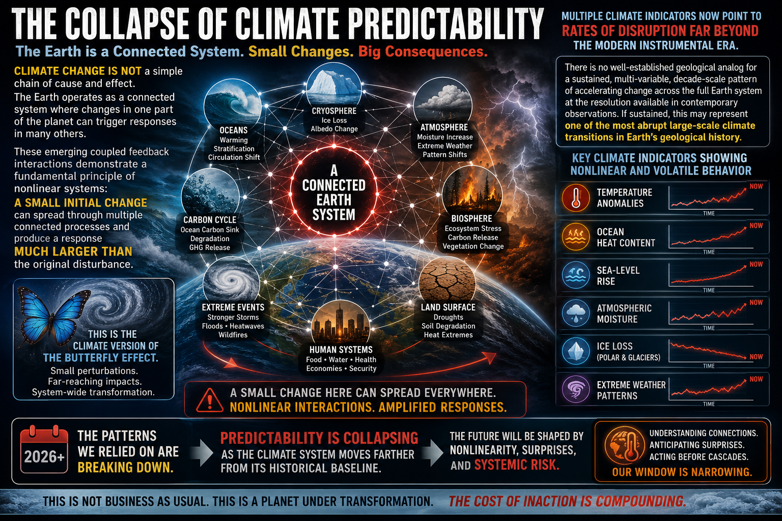
This transition is fundamentally a problem of nonlinear dynamics.

In linear systems:

  • responses are generally proportional to the forcing;
  • disturbances remain localized; and
  • historical relationships remain relatively stable.

In nonlinear systems:

  • small perturbations can produce disproportionately large responses;
  • interactions among multiple feedback loops amplify disturbances; and
  • outcomes become increasingly sensitive to initial conditions.

As climate systems become more strongly coupled, Earth’s behavior increasingly resembles a nonlinear network rather than a collection of independent oscillators.

This is the climate-scale manifestation of the Butterfly Effect.


Cascading Climate Responses

Once coupling strengthens sufficiently, climate events begin propagating across multiple systems.

For example:

Ocean Warming → Marine Heatwaves → Increased Evaporation → Higher Atmospheric Water Vapor → Stronger Atmospheric Rivers → Extreme Flooding → Reduced Snowpack → Earlier Runoff → Hotter Soils → Stronger Heat Domes → Additional Ocean Warming

Each step reinforces subsequent processes, creating cascading responses that are considerably larger than the original perturbation.


Beyond Traditional Climate Variability

Many recent extreme events have exceeded expectations based on historical climate statistics.

Persistent heat domes, multi-day atmospheric rivers, marine heatwaves, rapid intensification of tropical cyclones, widespread wildfire outbreaks, and simultaneous extremes occurring across multiple continents increasingly reflect the behavior of an interconnected system rather than isolated weather anomalies.

The climate is no longer responding solely through individual oscillations.

It is responding through interactions among oscillations.


A New Framework for Climate Science

Understanding future climate risk increasingly requires moving beyond analyses that focus on individual climate modes in isolation.

Future prediction will depend on understanding:

  • cross-basin ocean interactions;
  • atmospheric teleconnections;
  • cryosphere–ocean coupling;
  • biosphere–atmosphere feedbacks;
  • hydrologic amplification; and
  • nonlinear propagation through coupled climate networks.

The central scientific challenge is no longer identifying individual feedbacks, but understanding how those feedbacks interact simultaneously.


Conclusion

The growing accumulation of heat within Earth’s climate system is strengthening connections among atmospheric, oceanic, cryospheric, and biological processes. These interactions are transforming once largely independent climate oscillations into a coupled network of nonlinear feedbacks.

As coupling intensifies, disturbances spread more efficiently across the Earth system, historical relationships become less reliable, and extreme events increasingly exceed expectations derived from the past. The resulting decline in predictability is not evidence that the climate has become random. Rather, it reflects the behavior of a highly interconnected nonlinear system whose responses are increasingly governed by cascading interactions instead of isolated processes.

The collapse of climate predictability is therefore best understood not as the failure of climate science, but as the emergence of a new climatic regime—one in which understanding the connections between Earth’s major systems becomes as important as understanding the systems themselves.

bookmark_borderThe Evolution of the American Economy: Capitalism, State Capitalism, and Socialism

Introduction

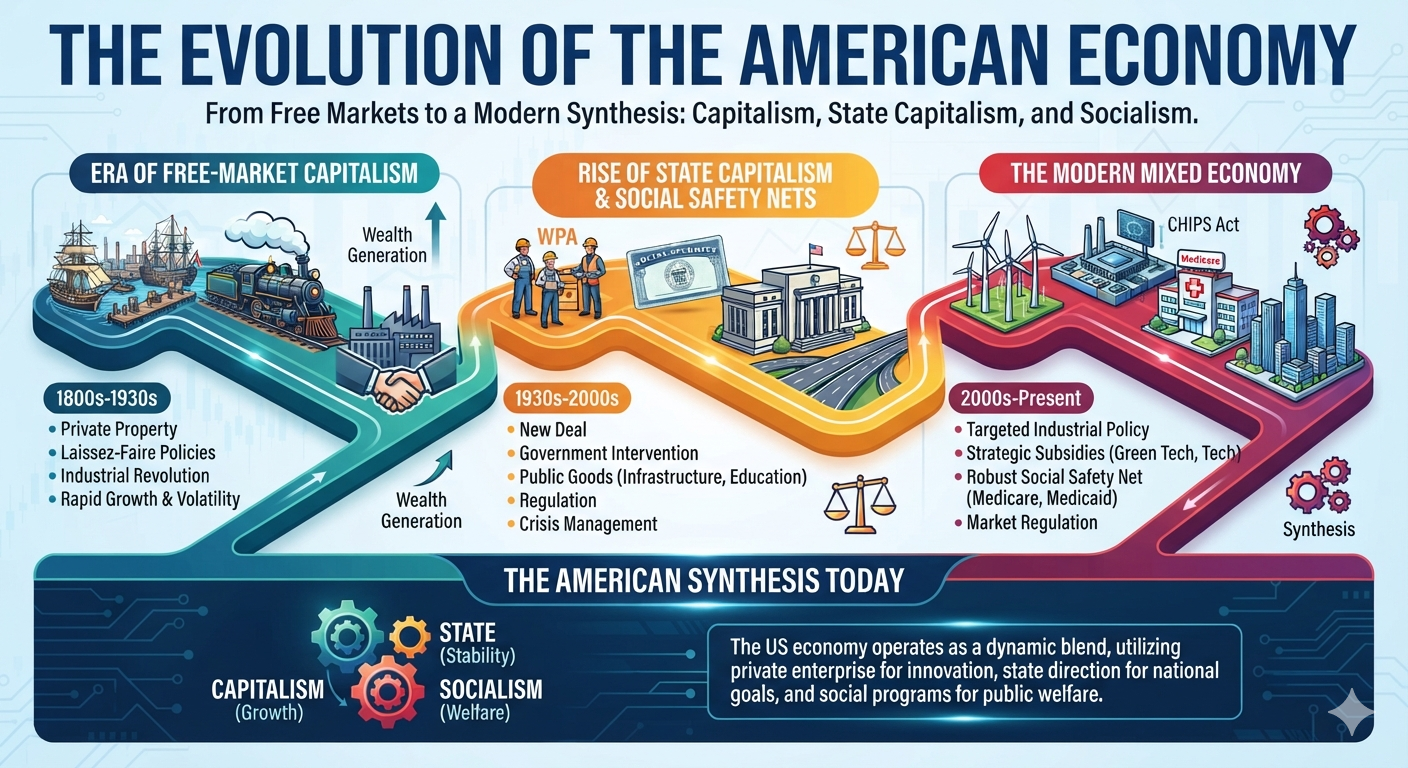
For much of its history, the United States has been portrayed as the world’s leading example of free-market capitalism, while socialism and communism have often been presented as fundamentally incompatible with American economic principles. In reality, no modern economy operates as a pure ideological model. Instead, governments continually adapt their economic policies in response to war, financial crises, technological competition, natural disasters, and changing national priorities.

Over the past several decades—and especially in recent years—the United States has significantly expanded the role of government in directing economic activity. Federal and state governments now provide targeted subsidies, acquire ownership stakes in private companies, shape investment decisions, guarantee markets for strategic industries, and assume financial risks that private markets are unwilling to bear. These policies are generally justified on the grounds of national security, economic competitiveness, supply-chain resilience, disaster recovery, or consumer protection.

This paper examines how these policies reflect characteristics traditionally associated with state-sponsored capitalism and socialism. Rather than arguing that the United States has abandoned capitalism, it demonstrates how the American economy has evolved into a hybrid system that combines free markets with substantial government intervention. Understanding this evolution provides important context for evaluating current economic policy and the changing relationship between government and private enterprise.

State-Sponsored Capitalism in the United States

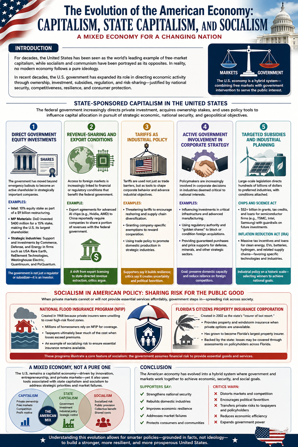
State-sponsored capitalism (also called state capitalism) refers to an economic system in which the government plays an increasingly active role in directing private investment, acquiring ownership stakes in companies, or using public policy to influence capital allocation in pursuit of strategic economic, national security, or geopolitical objectives.

In recent years, the United States has moved further toward this model. While market mechanisms remain the foundation of the U.S. economy, successive administrations have expanded the federal government’s role through direct investments, industrial policy, subsidies, export controls, tariffs, and other forms of intervention designed to strengthen domestic manufacturing, secure critical supply chains, and enhance national competitiveness.

The principal mechanisms through which the federal government has pursued state-sponsored capitalism include the following:

1. Direct Government Equity Investments

Historically, federal ownership of private corporations was generally limited to temporary emergency bailouts. More recently, however, the government has begun acquiring direct equity positions in strategically important companies.

Examples include:

  • Intel: The federal government obtained a 10% equity stake in Intel as part of a restructuring package that included approximately $9 billion in federal support.
  • MP Materials: The Department of Defense invested approximately $400 million to acquire a 15% ownership stake in MP Materials, making the federal government its largest shareholder while supporting domestic rare-earth mineral production.
  • Strategic Industries: Federal agencies, including the Departments of Commerce, Defense, and Energy, have supported or invested in companies involved in critical technologies and infrastructure, including USA Rare Earth, ReElement Technologies, Westinghouse Electric Corporation, Quantinuum, and PsiQuantum.

These investments represent a notable departure from traditional industrial policy by making the government not only a regulator and subsidizer, but also an investor.

2. Revenue-Sharing and Export Conditions

The federal government has increasingly linked access to export markets with financial or regulatory conditions.

One example is the export framework governing advanced artificial intelligence chips. Agreements allowing companies such as Nvidia and AMD to export certain AI processors to China have reportedly included provisions requiring companies to share a portion of the resulting revenues with the federal government. Critics, including analysts at the Cato Institute, argue that this approach resembles state-directed revenue extraction rather than conventional export licensing.

3. Tariffs as Industrial Policy

Tariffs have become an increasingly important instrument of industrial strategy.

Rather than functioning solely as broad trade barriers, tariffs have also been used to influence corporate behavior.

Examples include:

  • Threatening tariffs to encourage companies to relocate manufacturing or diversify supply chains.
  • Granting company-specific exemptions or adjustments that reward firms aligning with national industrial objectives.
  • Using trade policy to encourage domestic production in strategically important industries.

Supporters argue these measures strengthen national resilience, while critics contend they increase uncertainty and allow greater political influence over private investment decisions.

4. Active Government Involvement in Corporate Strategy

Federal policymakers have become increasingly involved in major corporate decisions affecting industries considered strategically important.

Examples include:

  • Influencing investment decisions involving critical infrastructure and advanced manufacturing.
  • Exercising regulatory authority to discourage foreign acquisitions of strategically important companies.
  • Employing “golden share” mechanisms or comparable government veto powers in selected transactions involving national security interests.
  • Providing guaranteed purchase agreements or price supports for defense-related technologies, critical minerals, and other strategic industries.

These policies seek to preserve domestic industrial capacity while reducing dependence on foreign suppliers.

5. Targeted Subsidies and Industrial Planning

The expansion of state involvement did not begin with direct government ownership. Earlier legislation established a broad framework for government-directed industrial policy through grants, tax incentives, loans, and regulatory requirements.

The CHIPS and Science Act

The CHIPS and Science Act committed more than $52 billion in grants, tax credits, and loan guarantees to expand domestic semiconductor manufacturing. Major beneficiaries include Intel, TSMC, Samsung, and other semiconductor producers.

Recipients were also subject to “guardrail” provisions limiting certain future investments in countries considered strategic competitors.

The Inflation Reduction Act (IRA)

The Inflation Reduction Act created extensive tax credits, grants, and financing mechanisms supporting renewable energy, electric vehicles, battery manufacturing, hydrogen production, and related supply chains.

The legislation represents one of the largest industrial policy initiatives in U.S. history, directing hundreds of billions of dollars toward technologies identified by policymakers as priorities for the energy transition.

A New Economic Model?

Taken together, these policies illustrate a significant evolution in the relationship between the federal government and private enterprise. Rather than relying primarily on market incentives and regulatory oversight, the government has increasingly acted as investor, financier, customer, shareholder, trade negotiator, and strategic planner.

Supporters argue that these interventions are necessary to compete with state-directed economies such as China, strengthen national security, rebuild domestic manufacturing, and secure critical supply chains.

Critics counter that expanding government ownership, selective subsidies, preferential treatment, and direct intervention in private markets blur the traditional distinction between free-market capitalism and state-sponsored capitalism. They warn that such policies may distort competition, encourage political favoritism, and reduce market efficiency.

Whether viewed as a pragmatic response to global competition or a fundamental shift in American economic philosophy, the growing role of the federal government in directing private capital represents one of the most consequential developments in U.S. economic policy in decades.

Socialism

One characteristic commonly associated with socialism is the government assuming responsibility for providing goods or services that private markets are unable or unwilling to provide. In these cases, financial risks and costs are shared across society through taxes, mandatory assessments, or publicly backed insurance programs.

The U.S. insurance industry provides several examples of this approach.

The National Flood Insurance Program (NFIP)

The National Flood Insurance Program (NFIP), administered by the Federal Emergency Management Agency (FEMA), was established in 1968 because private insurers were largely unwilling to provide affordable flood insurance in many high-risk areas.

Rather than leaving homeowners without coverage, the federal government assumed much of the financial risk. Today, millions of property owners purchase flood insurance through the NFIP, with taxpayers ultimately bearing a substantial portion of catastrophic losses when claims exceed collected premiums. The program illustrates how the government has socialized a specific category of insurance risk that the private market has historically struggled to insure profitably.

Florida’s Citizens Property Insurance Corporation

Florida provides one of the clearest state-level examples of government intervention in insurance markets.

The Citizens Property Insurance Corporation was created by the Florida Legislature in 2002 as a government-established, not-for-profit insurer intended to serve as the state’s “insurer of last resort.” Its purpose is to provide property and windstorm insurance for homeowners, condominium owners, renters, and businesses that cannot obtain comparable coverage from private insurers.

As hurricanes have become more destructive, litigation costs have risen, and many private insurers have reduced their exposure or exited the Florida market altogether, Citizens has expanded dramatically. What began as a safety net has evolved into Florida’s largest property insurer, covering well over one million policies.

Unlike a private insurance company operating solely for profit, Citizens is backed by the state. If claims substantially exceed its financial reserves, Florida law allows Citizens to levy assessments on many insurance policies throughout the state to help cover losses. In effect, the financial risk is spread broadly among policyholders rather than borne exclusively by the individual customers who file claims.

A Mixed Economic Model

Programs such as the National Flood Insurance Program and Citizens Property Insurance Corporation illustrate how the United States operates as a mixed economy rather than a purely laissez-faire capitalist system. When private markets fail to provide essential services at affordable prices, governments have often stepped in to provide financing, insurance, or direct support.

Supporters argue that these programs protect homeowners, stabilize housing markets, and ensure that essential insurance remains available despite increasing climate and catastrophe risks.

Critics contend that publicly backed insurance can distort market signals, encourage development in high-risk areas, and shift financial burdens from individual property owners to taxpayers or other policyholders.

Regardless of one’s perspective, these programs demonstrate that government assumption of economic risk—one characteristic often associated with socialist policies—has become an established component of the American insurance system while coexisting with a predominantly private-market economy.

Conclusion

The American economy has never been completely free of government intervention, but the scope and nature of that intervention have changed substantially over time. Today, federal and state governments influence private markets through direct ownership, industrial policy, targeted subsidies, publicly backed insurance programs, trade policy, regulatory oversight, and strategic investments. These policies increasingly resemble characteristics associated with state-sponsored capitalism, while programs such as federally backed flood insurance and state-run insurers illustrate elements commonly associated with socialized risk.

Supporters argue that these interventions strengthen national security, rebuild domestic manufacturing, improve economic resilience, and address market failures that private enterprise alone cannot solve. Critics contend that expanding government involvement can reduce market efficiency, distort competition, encourage political favoritism, and transfer private risks to taxpayers.

The United States remains a capitalist economy, but it is no longer accurately described as a purely laissez-faire one. Instead, it has evolved into a mixed economic system in which free markets coexist with significant government participation. Recognizing this reality allows for a more informed discussion of public policy—one based not on political labels, but on the practical ways governments and markets increasingly work together to shape economic outcomes.