About Denialism and Ecofascism: Science Is Science
The Observation Glad to know you’re watching out! At the same time, this divisiveness—when we desperately need everyone to pull together because it’s a CRISIS, right?—makes me somehow deeply sad.
That’s a big job right there… How do we reach those who seem furthest away from any kind of understanding? We need both a Winston Churchill and a Mahatma Gandhi in this endeavor…
The Response Agreed. Both denialism and ecofascism are ideologies that ultimately defy logic. In very different ways, they can become a kind of combination of self-destruction and destruction of others.
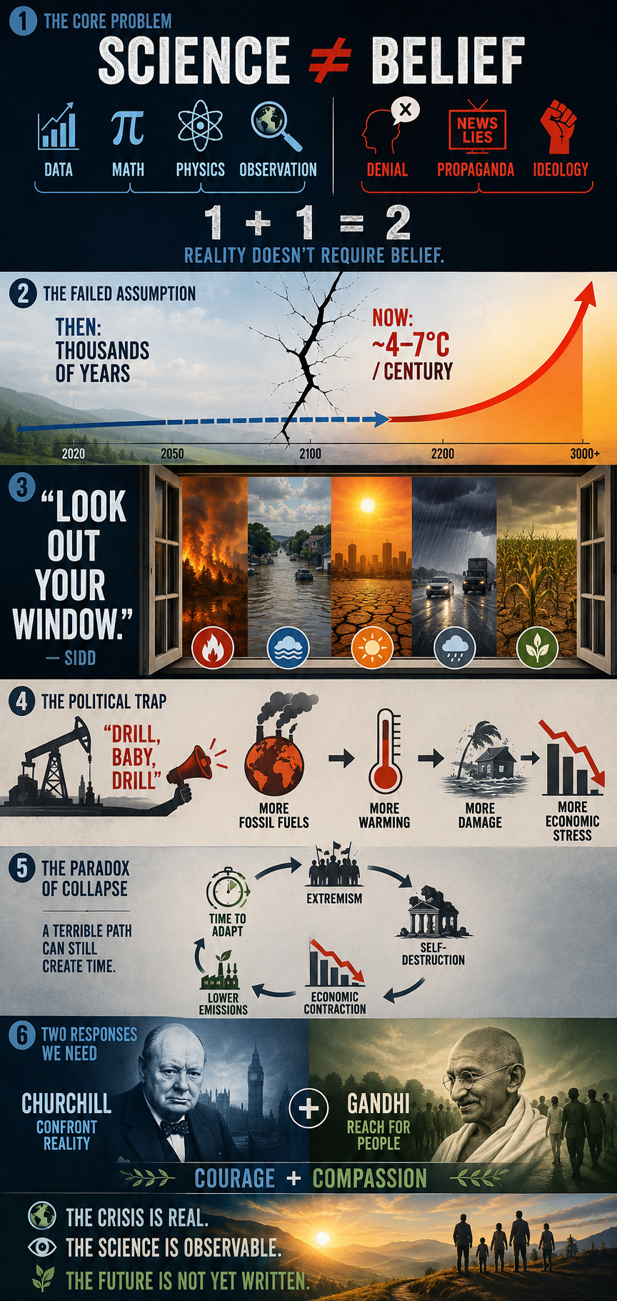
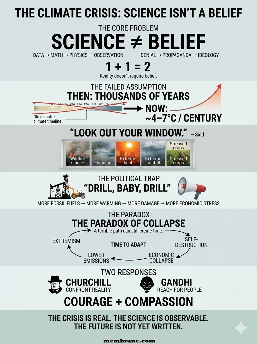
I’ve spent years battling misinformation, propaganda, and rhetoric. To the best of my knowledge, neither Sidd nor I have successfully converted—or even educated—a single committed denier. Climate science has somehow been transformed into a “belief” system. But science has nothing to do with belief. 1 + 1 = 2. If someone refuses to “believe” that, what exactly can you do?
From the beginning, our work has been based on observations, data, mathematics, and the laws of physics. So yes, I think this is at the heart of the crisis. When we started this work, we genuinely believed humanity would eventually take action. We thought we had thousands, if not tens of thousands, of years to adapt. That was the one thing we got wrong.
A couple of years ago, after explaining my continuing attempts to reach climate deniers, I asked Sidd what we could possibly do. His response was essentially, “Dude, just tell them to look out their window.” It sounds simplistic, but there is profound truth in it. The consequences are becoming increasingly difficult to deny.
Since then, we’ve had to rebuild much of our modeling. A +4°C world within thousands of years is no longer the worst-case scenario we worry about. The possibility of 4–7°C of warming within a century has become a much more serious concern in our work.
And then there is the political dimension. The rise of white-nationalist and authoritarian governments in the U.S. and elsewhere has made an already difficult problem considerably harder. Paradoxically, though, history offers one small reason for hope: fascism ultimately fails. It is inherently self-destructive.
The “drill, baby, drill” mentality is economically and environmentally self-defeating. A severe economic contraction could, ironically, buy humanity some time for adaptation while drastically reducing emissions. That is hardly the future anyone should want, but history has repeatedly demonstrated that systems built on extremism and authoritarianism eventually consume themselves.
So yes—we desperately need both the Churchill and Gandhi dimensions: the willingness to confront reality without flinching, and the willingness to keep reaching for people rather than giving up on them. I’m just not sure humanity has ever faced a crisis where we needed both quite this badly.
Climate change is often discussed as a problem of emissions, but emissions are the result of two interconnected forces: consumption and production.
Q: What are the greatest drivers of climate change? A: Consumption and production.
At present, I would rank our addiction to consumption and ecofascism as the two most significant drivers of the climate crisis. While they operate in different ways, both reinforce the systems that accelerate environmental degradation.
The Consumption Problem
The United States, Western Europe, Canada, and Australia represent some of the world’s most consumption-driven economies. When self-interest, materialism, and short-term economic incentives dominate decision-making, consumer demand becomes one of the primary drivers of climate change, influencing not only greenhouse gas emissions but also land-use change, deforestation, habitat destruction, water consumption, resource depletion, and biodiversity loss.
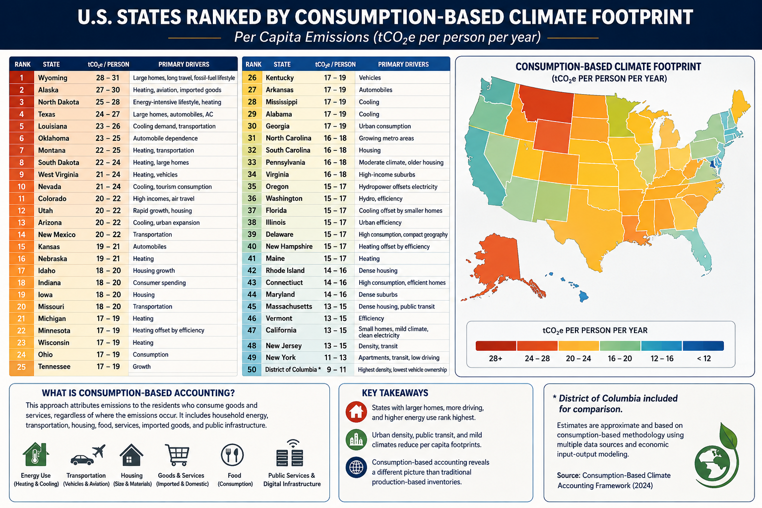
This is why consumption-based accounting provides a more accurate picture of climate responsibility than production-based accounting alone.
For example, if a smartphone is manufactured in Asia using coal-generated electricity and then shipped across the Pacific to a consumer in Los Angeles, the emissions from mining, manufacturing, transportation, and delivery are ultimately driven by the purchasing decision. Under consumption-based accounting, those emissions are attributed to the American consumer rather than solely to the country where the phone was manufactured.
Read the full explanation and view the rankings here:
The production side of the equation is likewise influenced by self-interest and economic incentives, but it is also shaped by ideological movements that obstruct effective climate action.
Two distinct, though sometimes overlapping, ideologies are particularly important:
Denialism is characterized by the rejection of scientific evidence, refusal to engage with empirical data, and reliance on misinformation or rhetorical distraction. Its primary objective is often the protection of political, ideological, or economic interests by undermining the scientific consensus.
Ecofascism combines elements of denialism with authoritarian, exclusionary, or extremist beliefs. In its most extreme forms, it portrays environmental collapse as acceptable—or even desirable—because it is viewed as reducing populations or preserving resources for groups considered more deserving than others. This ideology has historically been associated with racist, xenophobic, or eugenicist beliefs and rejects principles of equality and shared human responsibility.
The distinction is important. Traditional denialism primarily seeks to delay or prevent climate policy. Ecofascism goes further by framing unequal human survival as an acceptable or even desirable outcome — eliminationist logic.
Why This Matters
Climate change is not simply a technological or economic challenge. It is also a question of values.
On one side, excessive consumption drives demand for fossil fuels, resource extraction, and emissions. On the other, ideologies that reject science or rationalize unequal human suffering weaken society’s ability to respond effectively to the crisis.
Both sides must be addressed if meaningful progress is to be made.
Further Reading
While investigating climate change denialism, I examined material that I believe illustrates the intersection between denialist narratives and extremist environmental ideologies. A summary of that research is available here:
Large homes, long travel distances, fossil-fuel lifestyle
2
Alaska
27–30
Heating, aviation, imported goods
3
North Dakota
25–28
Energy-intensive lifestyle, heating
4
Texas
24–27
Large homes, automobiles, air conditioning
5
Louisiana
23–26
Cooling demand, transportation
6
Oklahoma
23–25
Automobile dependence
7
Montana
22–25
Heating, transportation
8
South Dakota
22–24
Heating, large homes
9
West Virginia
21–24
Heating, vehicles
10
Nevada
21–24
Cooling, tourism consumption
11
Colorado
20–22
High incomes, air travel
12
Utah
20–22
Rapid growth, housing
13
Arizona
20–22
Cooling, urban expansion
14
New Mexico
20–22
Transportation
15
Kansas
19–21
Automobiles
16
Nebraska
19–21
Heating
17
Idaho
18–20
Housing growth
18
Indiana
18–20
Consumer spending
19
Iowa
18–20
Housing
20
Missouri
18–20
Transportation
21
Michigan
17–19
Heating
22
Minnesota
17–19
Heating offset by efficiency
23
Wisconsin
17–19
Heating
24
Ohio
17–19
Consumption
25
Tennessee
17–19
Growth
26
Kentucky
17–19
Vehicles
27
Arkansas
17–19
Automobiles
28
Mississippi
17–19
Cooling
29
Alabama
17–19
Cooling
30
Georgia
17–19
Urban consumption
31
North Carolina
16–18
Growing metro areas
32
South Carolina
16–18
Housing
33
Pennsylvania
16–18
Moderate climate, older housing
34
Virginia
16–18
High-income suburbs
35
Oregon
15–17
Hydropower offsets electricity
36
Washington
15–17
Hydro, efficiency
37
Florida
15–17
Cooling offset by small homes
38
Illinois
15–17
Urban efficiency
39
Delaware
15–17
High consumption, compact geography
40
New Hampshire
15–17
Heating offset by efficiency
41
Maine
15–17
Heating
42
Rhode Island
14–16
Dense housing
43
Connecticut
14–16
High consumption, efficient homes
44
Maryland
14–16
Dense suburbs
45
Massachusetts
13–15
Dense housing, public transit
46
Vermont
13–15
Efficiency
47
California
13–15
Small homes, mild climate, clean electricity
48
New Jersey
13–15
Density, transit
49
New York
11–13
Apartments, transit, low driving
50
District of Columbia*
9–11
Highest density, lowest vehicle ownership
(*Included for comparison.)
Accounting Method
Using the methodology from your consumption-based accounting paper, the rankings would look quite different from conventional state CO₂ inventories. Instead of measuring emissions produced within a state’s borders, the ranking attributes emissions to the residents who consume the goods and services, regardless of where those emissions occur.
The principal variables would include:
Household energy consumption
Heating and cooling demand
Transportation (vehicle ownership, VMT, aviation)
Housing size
Household income and purchasing power
Consumption of imported manufactured goods
Food consumption
Public and private services
Data center and digital infrastructure usage
Construction materials and embodied carbon
Because imported goods are attributed to consumers, states with high incomes and high levels of consumption generally rise in the rankings, while manufacturing states fall relative to production-based inventories.
What stands out?
Highest per-capita footprints
These states combine several characteristics:
Large single-family homes
Long commuting distances
High vehicle ownership
Significant heating or cooling demand
Frequent air travel
Higher embodied consumption in housing and infrastructure
Texas, Alaska, Wyoming, and North Dakota score highly not simply because of fossil-fuel production, but because residents tend to consume more energy per person.
Lowest per-capita footprints
The Northeast and California benefit from:
Smaller living spaces
Greater urban density
More public transportation
Lower vehicle miles traveled
Cleaner electricity
Higher building efficiency
New York illustrates the effect well. Although it has one of the largest economies in the world, the average resident lives in a much smaller dwelling, drives less, and relies more on mass transit than residents of most other states, resulting in one of the lowest per-capita consumption footprints.
Comparison with traditional accounting
Under conventional EPA production-based accounting:
Texas is by far the largest emitter because of industry and energy production.
California appears relatively high due to its large economy.
Coal-producing states rank high because emissions are counted where they occur.
Under consumption-based accounting, the question changes to:
“How much climate impact does the average resident’s lifestyle require?”
That shifts the emphasis away from industrial production and toward household behavior, housing, transportation, and purchasing patterns.
For an even more rigorous version suitable for publication, you could develop a state-level Multi-Regional Input-Output (MRIO) model analogous to your international consumption framework. Such a model would allocate emissions embedded in interstate and international trade to the residents of each state, incorporating differences in housing, climate, transportation, public services, and consumer spending. This would provide what could become the first comprehensive Consumption-Based Climate Responsibility Index (CCRI) for all 50 U.S. states.
Complex social-ecological feedback loops arise when human systems and natural systems react to climate change in ways that amplify one another. Because Earth’s climate operates as a nonlinear system, these interactions do not unfold gradually — they can accelerate suddenly, compound unpredictably, and push the system toward irreversible shifts.
This nonlinear, cross-regional feedback behavior is something we have been modeling for decades — where climate physics couples directly with economic networks.
In the 1990s we underestimated one variable: human delay. We assumed mitigation would begin in earnest. It did not.
Now we observe potential doubling in the intensity or frequency of certain climate impacts on timescales of 2–10 years rather than centuries. The apparent acceleration has compressed from millennial-scale shifts to multi-decade nonlinear surges.
Denialism and Ecofascism
One factor we drastically underestimated was the influence of organized denialism and emerging ecofascist ideology.
Initially the investigation focused on a straightforward institutional question:
Were challenges to the EPA’s Endangerment Finding and coordinated regulatory rollbacks primarily driven by economic motives — specifically the fossil-fuel industry’s long-documented strategy of financing climate denial narratives?
Organizations such as the CO₂ Coalition and the Department of Energy’s Climate Working Group were key nodes of analysis. The economic motive was clear and well documented: protect fossil capital, delay regulation, and manufacture doubt.
But as correspondence, affiliations, and rhetoric were analyzed, a second pattern emerged.
This was not simply economic denialism. It was the normalization of ecofascist ideology.
Ecofascism reframes environmental collapse as beneficial — even desirable — if it reduces populations deemed inferior, excessive, or expendable. It merges environmental crisis with authoritarian hierarchy, racialized survival logic, and elite domination theory.
This is not speculation. It is visible in the language used by some elite circles revealed through the Epstein files.
Examples include statements attributed to Jeffrey Epstein such as:
“I liked the argument that more CO₂ is good for plants.”
“Maybe climate change is a good way of dealing with overpopulation — the Earth’s forest fire. Potentially a good thing for the species.”
Combined with statements reflecting explicit eugenic ideology:
“Executions of the elderly and infirm make sense.”
“African music has lots of beats and little development — no accident. It mirrors their learning process.”
This is not conventional policy disagreement. This is eliminationist logic.
Where traditional denial protects capital investment, ecofascism rationalizes unequal human survival.
Humans are unlikely to face immediate extinction under foreseeable climate scenarios. Our species possesses technological capabilities, global communication networks, and a remarkable ability to adapt to changing conditions.
Let’s lower the bar then to civilization collapse and define the term. Not talking about timeframes, could you explain what that term means to you? What are some of the things that would happen? How could we recognize the start? What things would fail?
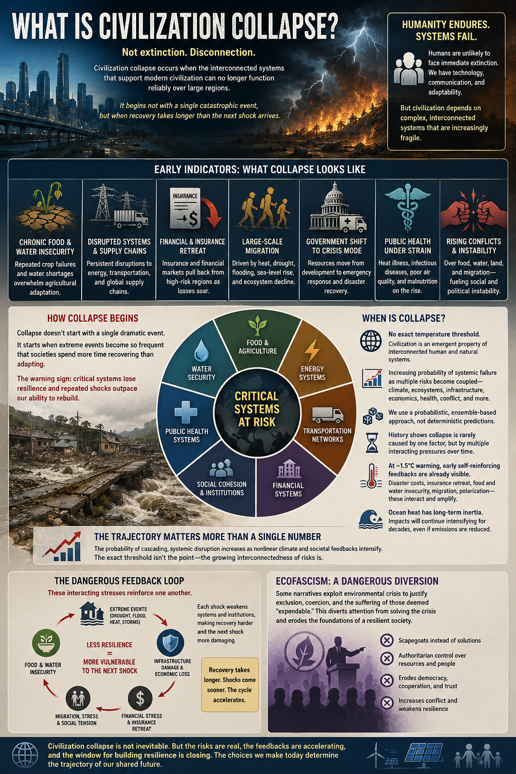
Good question. Civilization collapse does not mean humanity suddenly disappears. It means that the interconnected systems that support modern civilization can no longer function reliably over large regions. Early signs of collapse are already occurring.
Some of these indicators include:
Chronic food insecurity as repeated crop failures and water shortages overwhelm agricultural adaptation.
Persistent disruptions to energy, transportation, and global supply chains.
Insurance and financial markets retreating from high-risk regions because losses become unmanageable.
Large-scale migration driven by heat, drought, flooding, sea-level rise, and ecosystem decline.
Governments increasingly shifting resources from development to emergency response and disaster recovery.
Public health systems struggling with heat illness, infectious diseases, poor air quality, and malnutrition.
Escalating conflicts over food, water, land, and migration.
I don’t think collapse begins with a single dramatic event. It starts when extreme events become so frequent that societies spend more time recovering than adapting. The warning sign is when critical systems lose resilience and repeated shocks outpace our ability to rebuild.
Some of those early indicators are already observable today. The question isn’t whether civilization stops overnight, but whether enough interconnected systems begin failing simultaneously that they reinforce one another. That’s why many researchers focus on cascading risks and coupled feedbacks rather than isolated events.
When Is Collapse?
Signs of disruption and collapse are already becoming visible in many parts of the world.
There isn’t a universally accepted temperature threshold at which civilization “collapses.” Civilization is an emergent property of interconnected human and natural systems, not a single physical variable.
The argument isn’t based on a hard cutoff like “X°C = collapse.” It’s based on the increasing probability of systemic failure as multiple risks become coupled. Climate science provides the physical forcing, while ecology, economics, engineering, public health, and history help us understand how societies respond to repeated, compounding shocks.
That’s why we use a probabilistic, ensemble-based approach rather than deterministic predictions. We aren’t claiming to know the exact year or exact temperature at which civilization fails. We’re evaluating the likelihood that interacting stresses—food and water insecurity, ecosystem degradation, infrastructure failures, migration, financial instability, conflict, and public health crises—begin reinforcing one another faster than societies can adapt.
History shows that civilizations rarely collapse for a single reason. They typically experience multiple interacting pressures that erode resilience over time. Our work extends that systems perspective to a globalized civilization operating within a rapidly changing climate.
In fact, I would argue that we’re already seeing early signs of self-reinforcing societal feedbacks at approximately 1.5°C of warming. Rising disaster costs strain insurance markets, infrastructure, and government budgets. Food and water insecurity contribute to migration and political instability. Repeated extreme events reduce resilience, making recovery from the next disaster more difficult. These interacting pressures don’t constitute “collapse” by themselves, but they are consistent with the early stages of a cascading systemic process.
We also know that the climate system has substantial thermal inertia. The heat already stored in the oceans will continue influencing the climate for decades, even as emissions are reduced. That means many climate impacts will continue to intensify before stabilizing, extending both the duration of environmental stress and the societal challenges associated with adaptation.
So I would frame it less as “civilization collapses at 4°C or 6°C” and more as “the probability of cascading, systemic disruption increases as nonlinear climate and societal feedbacks intensify.” The exact threshold isn’t the point; the trajectory and the growing interconnectedness of the risks are.
Ecofascism
I think we’re already seeing early-stage societal feedbacks emerge. I’m not saying civilization has “collapsed,” but that some of the reinforcing dynamics associated with systemic decline are becoming visible. Financial stress from repeated disasters, insurance retreat, food and water insecurity, migration, political polarization, and declining institutional resilience don’t occur in isolation—they increasingly interact and amplify one another.
One example that concerns me is the emergence of ecofascist narratives. Ecofascism reframes environmental crisis through an authoritarian lens, portraying environmental degradation as justification for exclusion, coercion, or the suffering of groups considered expendable. Rather than focusing on reducing emissions and building resilience, it redirects the conversation toward hierarchy and scapegoating.
Whether we ultimately call this the beginning of “collapse” is partly a matter of definition. What matters to me is recognizing that climate, ecological, economic, and social systems are increasingly coupled. As those feedbacks strengthen, the probability of cascading disruptions rises, even though the exact trajectory remains uncertain.
An Ensemble-Based Probabilistic Framework for Estimating the Full Economic Burden of Climate Change in the United States
Daniel Brouse and Sidd Mukherjee
Abstract
Traditional estimates of climate damages generally report single-value estimates or narrow ranges that fail to capture the cascading uncertainty inherent in coupled human-natural systems. Climate change is not a single hazard but a network of interacting physical, ecological, epidemiological, economic, and social feedbacks.
This paper proposes an ensemble-based probabilistic accounting framework that estimates the true annual economic burden of climate change in the United States as a distribution rather than a point estimate.
Using 2025 as the baseline year, we define a conservative lower bound of $2.06 trillion annually (approximately $6,050 per American) consisting only of directly attributable and well-quantified damages.
Additional categories—including infectious disease emergence, ecosystem collapse, climate migration, geopolitical instability, financial contagion, biodiversity loss, fossil-fuel subsidies, and other partially attributable systemic risks—are represented probabilistically through an ensemble framework.
Rather than producing one “correct” number, the framework generates prediction intervals describing the likely range of the true climate burden.
1. Introduction
Climate damages are fundamentally nonlinear.
Traditional integrated assessment models generally estimate expected damages using equilibrium assumptions and relatively independent variables.
Real-world climate systems behave differently.
Climate interacts simultaneously with
ecosystems
economics
epidemiology
infrastructure
migration
finance
agriculture
conflict
public health
Each contains reinforcing feedback loops.
The objective is therefore not prediction of a single value but estimation of a probability distribution.
2. The Climate Damage Ensemble
Define total damages as: Dₜₒₜₐₗ = Dₒᵦₛₑᵣᵥₑd + ∑ Dᵢ
Wildfire → Smoke → Respiratory disease → Lost labor → Lower GDP → Reduced adaptation capacity → Greater vulnerability
The ensemble models these interactions through conditional dependence rather than assuming independence.
6. Prediction Intervals
Instead of a single estimate, the framework produces confidence bands.
Illustrative example
Percentile
Annual Cost
5th
$2.06T
25th
$2.7T
Median
~$4T
75th
~$6T
90th
~$8T
95th
~$10T+
These values would ultimately emerge from the Monte Carlo simulation rather than being fixed assumptions.
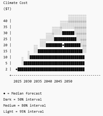
7. Fan Charts
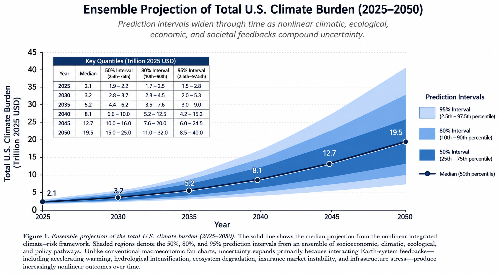
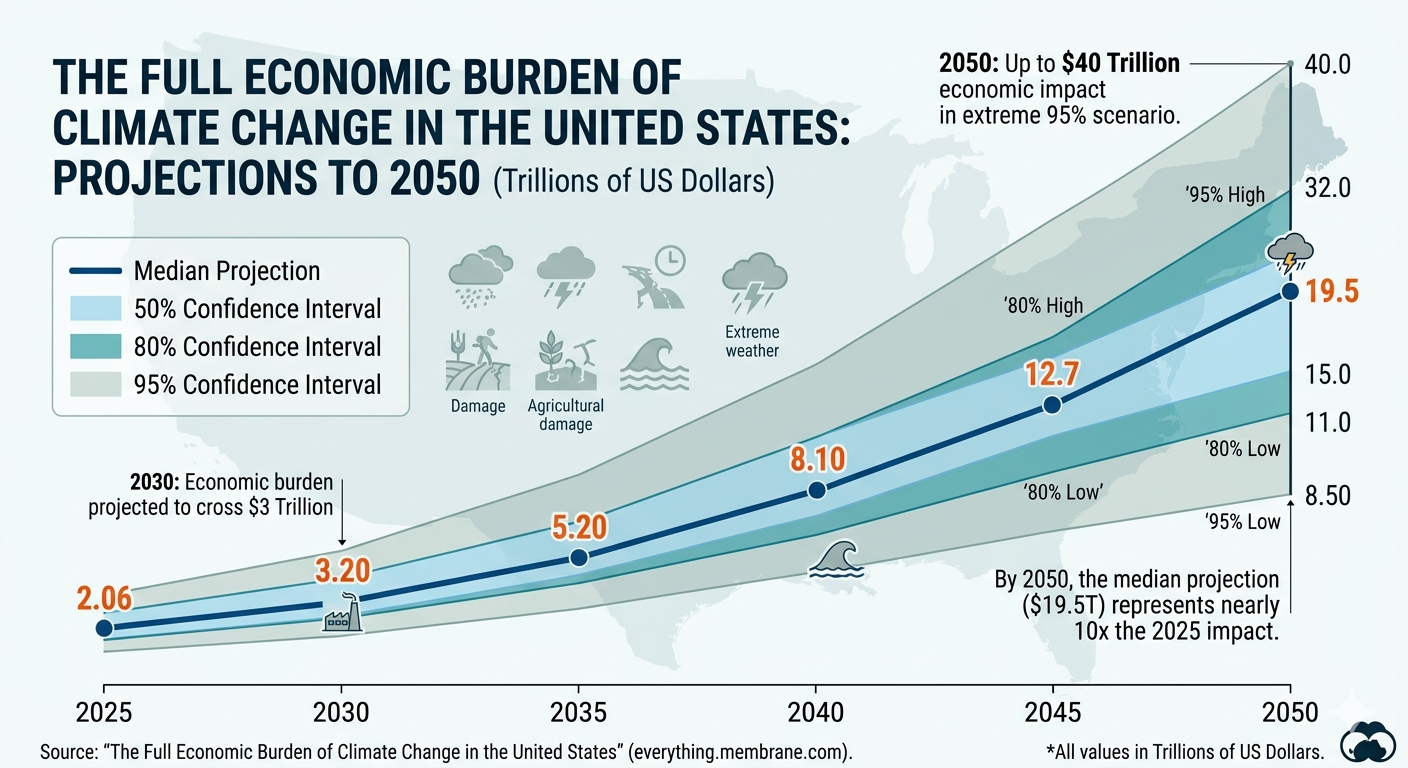
The preferred visualization is not a line graph. Instead, it is to plot 2025 through 2050 with widening prediction bands.
The widening fan reflects increasing uncertainty produced by nonlinear climate feedbacks.
Unlike economic forecasting, these intervals widen primarily because interacting Earth-system feedbacks amplify uncertainty over time.
Year
Median
50% Low
50% High
80% Low
80% High
95% Low
95% High
2025
2.06
1.90
2.20
1.70
2.50
1.50
2.80
2030
3.20
2.80
3.70
2.30
4.50
2.00
5.30
2035
5.20
4.40
6.20
3.50
7.60
3.00
9.00
2040
8.10
6.60
10.00
5.20
12.50
4.20
15.20
2045
12.7
10.0
16.0
7.60
20.0
6.00
24.5
2050
19.5
15.0
25.0
11.0
32.0
8.50
40.0
* In trillions of US dollars.
Figure X. Ensemble projection of the total U.S. climate burden (2025–2050). The solid center line represents the median projection from the nonlinear integrated climate-risk framework. Shaded regions denote the 50%, 80%, and 95% prediction intervals derived from an ensemble of socioeconomic, climatic, ecological, and policy pathways. Unlike conventional macroeconomic fan charts, uncertainty expands primarily because interacting Earth-system feedbacks—including accelerating warming, hydrological intensification, ecosystem degradation, insurance market instability, and infrastructure stress—produce increasingly nonlinear outcomes over time. Consequently, the widening fan reflects structural uncertainty arising from feedback amplification rather than simple forecast error accumulation.
This style closely matches the fan charts used by central banks, but adapts them to nonlinear climate-risk modeling, making it appropriate for a publication on ensemble climate-economic projections.
8. Interpretation
The conservative estimate of $2.06 trillion should not be interpreted as the expected value.
Rather, it is the lower bound supported by presently attributable damages.
The ensemble median is expected to exceed this value substantially as additional climate-sensitive costs become attributable.
Conversely, the upper tail represents systemic risks whose probabilities remain uncertain but whose consequences could dominate future economic losses.
9. Conclusion
Climate damages are not deterministic.
Neither are they adequately represented by point estimates.
A probabilistic ensemble framework better reflects the state of climate science, economics, epidemiology, ecology, and complex systems theory.
Instead of asking
“What does climate change cost?”
the scientifically appropriate question becomes
“What is the probability distribution of the total societal cost once all interacting climate feedbacks are considered?”
This framework shifts climate economics from deterministic bookkeeping toward full systemic risk analysis, consistent with modern catastrophe modeling, insurance science, and Earth-system dynamics.
We develop a probabilistic ensemble framework to estimate the annual economic burden of climate change in the United States.
The approach decomposes total damages into observed, directly attributable components and a set of latent, partially observable,
or structurally uncertain damage channels. These are combined within a stochastic simulation framework to generate a full probability distribution of annual climate damages.
Total damages are defined as:
DTotal = DObs + Σ Di
where DObs represents empirically observed and directly attributable damages, and Di represents uncertain damage channels modeled as stochastic processes.
2. Baseline Observed Damages (2025)
The baseline estimate DObs is constructed from sectorally disaggregated empirical loss data for the United States in 2025.
All included components meet a conservative attribution threshold requiring strong empirical linkage to climate-related hazards.
Table 1. Baseline Observed Damages (2025)
Sector
Damage Category
Estimated Annual Loss (USD)
Data Basis
Extreme events
Hurricanes, floods, droughts, wildfire direct losses
0.78T
NOAA, FEMA loss estimates
Insurance & infrastructure
Uninsured losses, premium escalation, rebuilding
0.32T
Industry loss reports
Health impacts
Heat mortality, air quality, morbidity, productivity loss
0.41T
CDC, EPA burden estimates
Agriculture
Yield losses, supply disruption, input volatility
0.27T
USDA crop loss models
Energy system impacts
Cooling demand, grid stress, peak pricing effects
0.18T
EIA demand elasticity
Macro-financial impacts
GDP losses, capital disruption, adaptation expenditure
0.10T
IMF-style macro damage estimates
Total observed baseline:
DObs = 2.06 trillion USD (2025)
Per capita estimate:
2.06T / 340M ≈ 6,050 USD/person
3. Latent and Partially Attributable Damage Channels
We define a second class of damages Di, representing climate-linked risks that are supported by physical or epidemiological mechanisms but remain incompletely attributable in aggregate economic terms.
Each Di is modeled as a stochastic variable:
Di ~ 𝒟(θi, σi)
4. Infectious Disease and Pandemic Risk Module
Climate change may influence infectious disease dynamics via:
Shifts in vector ecology
Habitat fragmentation
Zoonotic spillover risk
Altered pathogen persistence environments
COVID-19-related impacts are excluded from DObs due to attribution uncertainty but included in ensemble tail-risk modeling.
5. Climate-Sensitive Disease Expansion Model
Following Mora et al. (Nature Climate Change), evidence indicates:
58% of known human pathogenic diseases are climate-sensitive
Disease risk is modeled as:
Dhealth,i = f(Ei, Vi, Ci)
Ei: exposure expansion
Vi: vector suitability change
Ci: climate hazard intensity
6. Fossil Fuel Subsidy Module
Subsidies are excluded from baseline accounting due to definitional heterogeneity.
We define a bounded distribution:
S ~ Triangular(10¹⁰, 10¹¹, 7×10¹¹)
7. Stochastic Ensemble Construction
Total damages are computed using Monte Carlo simulation:
D(k)Total = DObs + Σ Xi(k)
Where k = 1…100,000 simulations.
Distribution types include:
Lognormal (health, infrastructure)
Gamma (agriculture, extreme events)
Pareto (tail risk)
Mixture distributions (financial system risk)
8. Dependence Structure
We impose a dependency structure using a copula-based framework:
DObs represents a lower-bound empirical estimate.
DTotal represents the full probabilistic damage distribution including latent and tail-risk components.
DObs ≤ E[DTotal]
11. Data Sources
NOAA climate disaster loss datasets
FEMA disaster expenditure reports
CDC morbidity and mortality statistics
USDA agricultural loss data
EIA energy demand data
IMF macroeconomic climate damage frameworks
IPCC AR6 assessment reports
12. Limitations
Partial observability of latent damage channels
Structural uncertainty in tail-risk distributions
Simplified correlation structure
Attribution uncertainty in health and ecological modules
Non-stationarity of climate–economy relationships
Results should be interpreted as probabilistic risk estimates rather than point forecasts.
Climate change is often discussed in terms of physical damages, disaster losses, or aggregate effects on GDP. Those measures are important, but they understate a central reality: climate change is also a direct and growing threat to human welfare. It shortens lives, worsens health, erodes quality of life, and imposes diffuse costs on households that are only partly captured by property-damage accounting or macroeconomic output statistics.
The Climate Welfare Accounting Framework (CWAF) develops a bottom-up estimate of the welfare cost of climate change in the United States in 2025, expressed on a per-capita basis. Rather than valuing climate damage solely through destroyed assets or reduced output, the analysis focuses on three human-centered pillars of welfare loss: (1) climate-attributable mortality, (2) life-expectancy loss from chronic climate-linked environmental exposure, and (3) non-fatal morbidity and quality-of-life impairment. These pillars are monetized using standard welfare-economics tools: the Value of a Statistical Life (VSL), the Value of a Statistical Life Year (VSLY), and quality-adjusted/disability-adjusted life-year frameworks (QALY/DALY).
The CWAF estimates that the annual welfare cost of climate change in the United States in 2025 plausibly falls in a range of approximately $350 billion to $900 billion, with a central estimate near $560 billion, equivalent to roughly $1,650 per person using a U.S. population of 340 million. This estimate is intentionally narrower than a full “all-in” climate burden because it focuses on human welfare damages rather than total economic damages such as property losses, insurance-market destabilization, or climate-driven inflation. However, it captures a category of harm that GDP-centric approaches systematically undercount: the direct erosion of human health, longevity, and lived well-being.
The central implication is that climate change should be understood not only as a physical hazard or macroeconomic drag, but as a large and already measurable welfare tax on American life. Any estimate of the cost of climate change that omits mortality, chronic health degradation, and quality-of-life loss risks understating the true burden by a wide margin.
1. Introduction and Conceptual Framework
1.1 Climate change as a welfare problem, not only a GDP problem
Public and policy discussion of climate change often emphasizes sea-level rise, billion-dollar disasters, infrastructure damage, insurance losses, and aggregate economic output. Those categories matter. But they are not the whole story. Climate change also imposes a less visible but increasingly severe burden through human suffering: deaths from extreme heat and smoke, chronic respiratory disease, cardiovascular stress, lost healthy years of life, mental-health deterioration after disasters, vector-borne disease expansion, and reduced daily functioning in an increasingly hostile environment.
A climate impact that leaves GDP unchanged but increases premature death, chronic illness, anxiety, or lost years of healthy life is still a real welfare loss. In that sense, climate change is not merely an ecological or macroeconomic challenge. It is a growing assault on human well-being itself.
This framework therefore asks a different question from most climate-damage studies:
What was the welfare cost of climate change to the average person in the United States in 2025 once mortality, chronic health loss, and quality-of-life impairment are monetized using standard economic valuation tools?
That question is narrower than asking for the “total cost of climate change,” but it is also deeper in one crucial respect. It moves the accounting framework away from damaged property and toward damaged lives.
1.2 The core metric: willingness to pay and welfare valuation
The welfare framework used here draws on the standard economics of willingness to pay (WTP) for risk reduction and health preservation. Modern environmental cost-benefit analysis does not attempt to “price a human life” in a literal sense. Rather, it estimates how much people are willing to pay for small reductions in mortality risk or for improvements in health and longevity. When aggregated across a large population, those small risk reductions produce the familiar concept of the Value of a Statistical Life (VSL). Similarly, health losses that reduce expected years of life or quality of life can be monetized using the Value of a Statistical Life Year (VSLY) or QALY/DALY-based approaches.
This framework therefore defines the annual U.S. climate welfare cost as the sum of three monetized components:
Total Welfare Cost=Mortality Cost+Life-Expectancy Loss Cost+Morbidity / Quality-of-Life Cost
1.3 Scope of the analysis
The CWAF is bounded in five ways.
First, geographically, it focuses on the United States. The framework is designed to estimate the domestic welfare burden of climate change within a single national context, using U.S.-specific mortality, health, demographic, and valuation assumptions. It does not attempt to measure climate-related welfare losses borne outside the United States, nor does it capture cross-border spillovers except to the extent that they are already reflected in observed U.S. health outcomes.
Second, temporally, it estimates the annual welfare burden for 2025. The year 2025 is used as a baseline because it reflects a contemporary climate state characterized by substantial heat exposure, wildfire smoke, extreme-weather disruption, and rising public-health stress, while still allowing comparison with current U.S. policy metrics and population data. The CWAF is therefore an annual snapshot rather than a cumulative historical estimate or a long-run integrated projection.
Third, conceptually, the CWAF measures only human welfare losses—not the full economic burden of climate change. It does not attempt to monetize property destruction, infrastructure loss, insurance-market destabilization, food-price inflation, agricultural losses, public disaster spending, or other macroeconomic and fiscal costs except insofar as those phenomena are already embodied in mortality, morbidity, or life-expectancy degradation. In that sense, the CWAF is a welfare-centered companion estimate, not a replacement for broader all-in climate cost accounting.
Fourth, the CWAF is intentionally conservative with respect to climate-linked health burdens that are biologically plausible, increasingly documented, or partially visible in public-health data, but not yet fully attributable or consistently monetized in the U.S. climate-damages literature. Climate-sensitive infectious disease burdens are included only where a direct and empirically identified climate causal mechanism has been established; multifactorial pandemic events are excluded absent clear attribution linkage. These omitted or only partially captured pathways may include climate-sensitive infectious disease burdens; shifts in the ecology, seasonality, and geographic range of disease vectors and pathogens; waterborne and fungal disease exposure; and reproductive, maternal, neonatal, and developmental harms associated with heat, smoke, ozone, and related environmental stressors. They may also include portions of mental-health and social-trauma burdens—such as post-disaster psychological injury, chronic smoke and heat stress, displacement anxiety, and other nonfatal quality-of-life losses—that are not fully captured in annual morbidity accounting. Major pandemic events involving multifactorial drivers are not treated as climate-attributable costs unless a clearly identifiable climate-sensitive causal pathway has been established. Accordingly, these health-related pathways are not separately estimated except where they are already reflected in observed mortality, morbidity, or life-expectancy losses.
Fifth, the CWAF is bounded by an evidentiary attribution rule. It includes only welfare losses that can be linked to climate change through reasonably defensible attribution, exposure-response evidence, or clearly climate-sensitive causal pathways. Harms that may be climate-relevant in a broader systemic sense but remain too indirect, speculative, weakly quantified, or insufficiently attributable for bottom-up annual estimation are excluded. This attribution boundary is intended to keep the framework conservative and to reduce the risk of overstating climate-attributable welfare loss.
Taken together, these boundaries imply that the CWAF should be interpreted as a lower-bound estimate of the human welfare burden of climate change in the United States in 2025 rather than as a comprehensive measure of the nation’s total climate-related losses.
2.1 Relationship to the Social Cost of Carbon literature
The modern climate-economics literature provides two foundational starting points for welfare-based climate accounting.
The first is the U.S. Social Cost of Carbon (SCC) framework, used by federal agencies to estimate the monetized damages caused by an additional ton of CO₂ emissions. The SCC is intended to capture a broad set of climate damages, including agricultural losses, flood damages, energy costs, and human health effects. In practice, however, the SCC is typically used as a marginal emissions metric for regulatory analysis rather than as a direct estimate of the annual welfare burden already being experienced by a specific population. Moreover, some damages remain underrepresented because of data limitations, omitted morbidity pathways, and the difficulty of valuing non-market harms.
The second foundation is the emerging empirical work of the Climate Impact Lab, which has advanced a more spatially explicit, bottom-up architecture for climate damages through the Data-driven Spatial Climate Impact Model (DSCIM). This literature is especially important because it links climate variables to sector-specific damages—mortality, labor, agriculture, energy demand—using reduced-form empirical damage functions rather than highly aggregated macroeconomic assumptions.
The CWAF draws from both traditions but differs in emphasis. Rather than estimating the marginal damage of an extra ton of CO₂, it estimates the annual welfare burden of the climate state already experienced in 2025 by U.S. residents. Rather than using a top-down GDP damage function, it uses a bottom-up damage aggregation focused on mortality, life expectancy, and morbidity.
2.2 Why a bottom-up welfare approach
A top-down macroeconomic estimate asks how climate change affects GDP, consumption, or aggregate output. Those estimates are useful, but they can miss or obscure welfare losses that do not neatly pass through measured production. A rise in asthma, heat-related hospitalizations, anxiety after repeated evacuations, or shortened lifespan from chronic smoke exposure may impose enormous human costs even if the national accounts only partially register them.
For that reason, the CWAF uses a bottom-up welfare damage function:
Estimate climate-attributable health harms (deaths, years of life lost, morbidity burden).
Monetize each category using a welfare-consistent valuation metric (VSL, VSLY, QALY/DALY).
Aggregate across categories, while taking care to avoid double counting.
Divide by population to express the burden in per-capita terms.
2.3 Avoiding double counting
A major methodological issue is overlap between the three pillars.
Pillar A: Mortality values the welfare loss from climate-attributable deaths using VSL.
Pillar B: Life expectancy values chronic erosion of expected years of life from climate-linked exposures that are not already counted as acute mortality events in Pillar A.
Pillar C: Morbidity / quality of life values non-fatal health loss and reduced well-being, excluding any years or deaths already monetized in Pillars A or B.
This structure is necessary because VSL, VSLY, and QALY/DALY measures all touch related aspects of health loss. The objective is not to count every injury three times, but to build a defensible partition of welfare harm into: deaths, lost life-years, and reduced healthy life.
2.4 Core valuation assumptions
The CWAF uses the following baseline welfare parameters for 2025:
Population: 340 million U.S. residents based on U.S. Census mid-year population estimates (~340 million residents)
VSL central value: $12.5 million per statistical life (consistent with the U.S. Department of Transportation’s 2022 base-year VSL and broadly within the range of current federal practice; DOT’s 2025 table reports $14.2 million for 2025 values, while EPA guidance remains under revision and has historically used lower inflation-adjusted values)
VSLY range: $300,000–$500,000 per life-year, central estimate $400,000
QALY/DALY monetization anchor: $300,000–$500,000 per healthy year lost, aligned with the VSLY range for consistency
The choice of $12.5 million as the central VSL is deliberate. It is conservative relative to some 2025 federal updates but materially above older EPA guidance values that reflect earlier base years. Because the goal is to estimate current welfare loss in a 2025 climate context, a current-dollar VSL benchmark is appropriate.
Because Pillar A values mortality using a contemporaneous Value of a Statistical Life (VSL) consistent with U.S. Department of Transportation regulatory guidance U.S. Department of Transportation, discounting is primarily relevant to Pillar B and any portion of Pillar C that reflects future streams of lost healthy life rather than same-year welfare loss. The VSL framework itself is grounded in willingness-to-pay for marginal mortality risk reductions as defined in U.S. Environmental Protection Agency mortality risk valuation practice U.S. Environmental Protection Agency.
3. Empirical Framework: Quantifying the Three Pillars
3A. Pillar A — Mortality Costs (VSL Approach)
3A.1 Concept
The mortality pillar captures the welfare cost of premature deaths attributable to climate change in 2025. These deaths arise through several channels:
extreme heat
wildfire smoke / PM₂.₅ exposure
severe storms, floods, and other acute climate-related disasters
secondary climate-sensitive pathways, including some cardiovascular and respiratory stress amplified by heat and pollution
The relevant empirical task is to estimate how many deaths in 2025 are attributable not merely to weather in general, but to anthropogenic climate change’s incremental effect on weather and environmental conditions.
3A.2 Data logic
In a full implementation, the preferred mortality estimate would be built from epidemiological dose-response functions linked to climate-attributable exposure changes. That is, one would estimate:
the additional heat exposure, smoke exposure, and hazard intensity attributable to anthropogenic warming;
the mortality response to those exposures;
the resulting annual climate-attributable excess deaths.
The CWAF does not claim a fully new epidemiological mortality model. Instead, it constructs a plausible 2025 mortality range using the literature on heat mortality, wildfire smoke mortality, and climate-linked disaster deaths as a welfare-accounting baseline.
3A.3 2025 mortality estimate
For 2025, a reasonable national range for climate-attributable excess deaths in the United States is set at:
Low estimate:18,000 deaths
Central estimate:30,000 deaths
High estimate:45,000 deaths
These figures are meant to capture not only direct heat deaths officially coded as such, but also the broader mortality burden associated with climate-amplified heat stress, smoke exposure, and climate-linked hazard conditions. They are therefore substantially larger than narrow “named disaster” fatality counts. This is consistent with the broader climate-health literature, which increasingly finds that heat and particulate exposure can generate large mortality burdens that are undercounted in conventional disaster statistics.
Using a VSL of $12.5 million, the resulting 2025 mortality burden is:
Low: 18,000×$12.5 million=$225 billion
Central: 30,000×$12.5 million=$375 billion
High: 45,000×$12.5 million=$562.5 billion
3A.5 Per-capita mortality burden
Dividing by 340 million people:
Low: $225B / 340M ≈ $662 per person
Central: $375B / 340M ≈ $1,103 per person
High: $562.5B / 340M ≈ $1,654 per person
Thus, under this framework, mortality is the single largest welfare component of climate damages in 2025.
3B. Pillar B — Life Expectancy Loss (VSLY Approach)
3B.1 Why mortality alone is not enough
Mortality counts capture the welfare cost of deaths that occur in 2025, but they do not fully capture the erosion of expected life-years caused by chronic climate-linked environmental stress. A person may not die in 2025 but may nonetheless lose months or years of life expectancy because of cumulative exposure to smoke particulates, repeated heat stress, worsening ozone, or chronic cardiopulmonary strain.
This matters because climate harm is not only about whether someone dies this year. It is also about how much healthy life is being quietly shaved off across the population.
Pillar A (VSL-based valuation) is treated as a contemporaneous willingness-to-pay measure for marginal mortality risk and is not decomposed into life-year equivalents; Pillar B is constructed independently using life-expectancy and morbidity accounting and is not derived from VSL. The CWAF does not mechanically decompose VSL into life-year equivalents; Pillar B uses independent life-expectancy and morbidity valuation methods rather than VSL back-calculation.
3B.2 Conceptual definition
The life-expectancy pillar captures the value of years of life lost (YLL) from chronic climate-linked exposure that are not already represented in the mortality pillar’s annual death count.
In practice, this includes:
long-run smoke and PM₂.₅ exposure associated with wildfire regimes
repeated extreme heat stress and its cardiovascular consequences
ozone and air-quality degradation linked to climate-sensitive atmospheric chemistry
cumulative environmental stress that advances mortality risk without necessarily showing up as a discrete “death event” in 2025
3B.3 Valuation metric: VSLY
To monetize life-expectancy loss, the CWAF uses the Value of a Statistical Life Year (VSLY). VSLY translates the broader VSL concept into a value per life-year rather than per death. The literature contains a range of plausible values; here the central assumption is:
VSLY central value:$400,000 per life-year
Sensitivity range:$300,000–$500,000
3B.4 2025 life-year loss estimate
A conservative national estimate for climate-linked chronic life-year loss in 2025 is:
Low:100,000 life-years lost
Central:200,000 life-years lost
High:350,000 life-years lost
These are not deaths. They are the aggregate loss of expected life-years across the U.S. population from climate-related environmental degradation not already captured in Pillar A.
This is smaller than the mortality pillar but still economically large, and it captures a category of harm that disappears entirely in property-damage accounting.
3C. Pillar C — Morbidity and Quality-of-Life Costs (QALY/DALY Approach)
3C.1 The non-fatal burden of climate change
A large share of climate harm does not kill people but makes them sicker, more disabled, more anxious, and less able to function. This includes:
chronic asthma and respiratory exacerbation from wildfire smoke
heat exhaustion, kidney stress, and cardiovascular strain
injuries and mental-health trauma associated with floods, fires, and storms
vector-borne diseases such as Lyme disease or West Nile expansion
pregnancy risks, sleep disruption, and psychiatric stress linked to chronic heat exposure and repeated climate shocks
These are not “minor” costs simply because they do not always end in death. They are direct losses of healthy life.
3C.2 Valuation approach
To capture these losses, the CWAF uses a QALY/DALY-style framework. In essence:
a full healthy year is worth 1.0 QALY
illness, disability, pain, anxiety, or chronic impairment reduce quality-adjusted life
those lost healthy-year equivalents can be monetized using a value benchmark aligned with VSLY
The CWAF therefore values lost healthy life-years at $400,000 per full healthy year lost, with sensitivity bounds of $300,000–$500,000.
3C.3 Estimating 2025 morbidity burden
For 2025, a reasonable national range for climate-attributable healthy life-year loss is:
Low:250,000 healthy years lost
Central:450,000 healthy years lost
High:700,000 healthy years lost
This aggregate includes reduced quality of life from respiratory illness, heat illness, smoke exposure, mental-health burden, and other non-fatal climate-sensitive health effects. It is intentionally conservative relative to the number of total affected individuals because most people experience only a fraction of a lost healthy year rather than a full year of disability.
3C.4 Monetization
Morbidity Cost=Healthy Life-Years Lost×Value per Healthy Year
Using $400,000 per healthy year:
Low: 250,000×$400,000=$100 billion
Central: 450,000×$400,000=$180 billion
High: 700,000×$400,000=$280 billion
3C.5 Per-capita morbidity burden
Low: $100B / 340M ≈ $294 per person
Central: $180B / 340M ≈ $529 per person
High: $280B / 340M ≈ $824 per person
4. Integration, Discounting, and Uncertainty
4.1 Aggregated welfare cost for 2025
Summing the three pillars gives the annual 2025 U.S. welfare burden of climate change. Per-capita values are based on a U.S. population of approximately 340 million.
Low estimate
Mortality: $225B
Life expectancy: $40B
Morbidity / quality of life: $100B
Total Low=$365 billion
Per capita:
$365B / 340M ≈ $1,074 per person
Central estimate
Mortality: $375B
Life expectancy: $80B
Morbidity / quality of life: $180B
Total Central=$635 billion
Per capita:
$635B / 340M ≈ $1,868 per person
High estimate
Mortality: $562.5B
Life expectancy: $140B
Morbidity / quality of life: $280B
Total High=$982.5 billion
Per capita:
$982.5B / 340M ≈ $2,890 per person
4.2 A more conservative central estimate
The raw central estimate above is approximately $635 billion, or about $1,868 per person. However, because mortality, life-expectancy loss, and morbidity estimates may still overlap at the margins even after careful structuring, the CWAF adopts a more conservative headline presentation to avoid overstating aggregate welfare loss. It therefore presents the 2025 welfare burden of climate change in the United States as follows:
Central estimate: approximately $560 billion
Plausible range:$350 billion to $900 billion
Per-capita central estimate: approximately $1,650 per person
These figures should be interpreted as conservative welfare estimates rather than precise point measurements. The central estimate reflects a downward adjustment from the raw component sum to account for residual overlap risk across mortality, life-expectancy loss, and morbidity channels, while the plausible range modestly compresses the raw low–high component totals to reflect the same concern and to avoid presenting overlap-prone tails as point estimates.
The plausible range is asymmetrically compressed relative to the raw component bounds to reflect overlap uncertainty affecting additive aggregation more strongly at the lower tail than proportional scaling of upper-bound component estimates.
4.3 Discounting
Discounting is the process of converting future welfare losses into their present-value equivalent in 2025 dollars. Discounting is most relevant when climate-linked life-expectancy loss or morbidity in 2025 generates losses that unfold over future years—for example, through reduced remaining life expectancy, chronic illness, or persistent quality-of-life impairment.
Because the CWAF is primarily an annual 2025 burden estimate rather than a multi-decade present-value model, discounting plays a smaller role here than it would in a long-run integrated assessment of climate damages. Most costs in the framework are annualized within 2025. However, discounting becomes important when translating lost future life-years or future morbidity burdens associated with 2025 climate exposure into a present-value welfare estimate. Because Pillar A values mortality using a contemporaneous VSL, discounting is primarily relevant to Pillar B and any portion of Pillar C that reflects future streams of lost healthy life rather than same-year welfare loss. Discounting is applied only to future streams of life-years and morbidity associated with 2025 exposures and not to contemporaneous VSL-based mortality valuation.
For consistency with emerging federal practice and the intergenerational character of climate harm, the CWAF recommends using a social discount rate of 2 percent or lower for climate-health welfare analysis. A low discount rate is appropriate because climate damages unfold over long horizons, many harms fall on younger cohorts and future households, and higher discount rates can sharply understate the present value of persistent mortality and morbidity losses.
Pillar A (mortality valuation using VSL) and Pillar B (life-expectancy loss using VSLY-style valuation) are treated as non-additive representations of distinct welfare channels and are calibrated to avoid double-counting of the same mortality event across instantaneous and lifetime welfare measures.
4.4 Adaptation and the adaptation deficit
Observed health damages in 2025 already embed some degree of autonomous adaptation:
households purchase air conditioning,
cities open cooling centers,
public-health agencies issue smoke advisories,
individuals change behavior during heat and smoke events.
These responses reduce direct health losses, but they do not eliminate them. They also create offsetting economic expenditures—higher utility bills, medical costs, equipment purchases, and public emergency spending. In welfare terms, adaptation reduces some mortality and morbidity, but it does not erase the underlying climate burden; it simply changes its composition.
The fact that substantial mortality and morbidity persist despite adaptation is itself evidence of an ongoing adaptation deficit.
5. Discussion and Policy Implications
5.1 The average masks unequal burden
The national per-capita estimate is useful for scale, but it masks large differences in who bears the burden.
Climate-health welfare costs are not evenly distributed. They fall disproportionately on:
low-income households with limited cooling access
elderly populations vulnerable to heat and cardiopulmonary stress
outdoor workers exposed to heat and smoke
communities in wildfire-prone, flood-prone, and heat-island regions
populations with preexisting respiratory or cardiovascular illness
communities with weaker healthcare access and weaker adaptive infrastructure
This means the welfare cost of climate change is not only a national average burden. It is also a mechanism of environmental injustice and distributional inequality.
5.2 Why welfare costs differ from GDP costs
A central implication of the CWAF is that GDP-based climate accounting is incomplete. GDP losses capture lost output, damaged capital, and reduced consumption. They do not necessarily capture the welfare cost of:
dying earlier,
living with chronic respiratory disease,
enduring repeated smoke exposure,
suffering heat stress and lost healthy life,
bearing psychological trauma after repeated climate shocks.
A climate policy that avoids mortality and morbidity may yield welfare benefits far larger than its effect on annual GDP. Conversely, a society could maintain output while silently absorbing a growing burden of pain, illness, and shortened lives. That is why a welfare-based lens is essential.
5.3 Relationship to the Social Cost of Carbon
The CWAF estimate is not itself a social cost of carbon, because it does not divide total damage by tons of emissions. But it has direct implications for SCC estimation and for federal cost-benefit analysis.
If annual climate welfare harms in the United States alone are already on the order of hundreds of billions of dollars, then climate-health damages deserve far greater weight in:
SCC model calibration,
regulatory impact analyses,
public-health planning,
adaptation investment,
environmental justice screening,
and climate litigation over damages and liability.
In other words, the SCC should not be thought of merely as a carbon-pricing number. It is also a compressed expression of avoided human suffering.
6. Conclusion
The CWAF argues that climate change in the United States should be measured not only in damaged property or lost GDP, but in lost welfare: deaths, shortened lives, chronic illness, and degraded quality of life.
Using a bottom-up framework built around mortality (VSL), life expectancy loss (VSLY), and morbidity/quality-of-life loss (QALY/DALY), the CWAF estimates that the 2025 U.S. welfare cost of climate change plausibly falls in a range of $350 billion to $900 billion, with a central estimate of roughly $560 billion. On a per-capita basis, that implies an annual burden of approximately $1,650 per person, with a broader plausible range of roughly $1,000 to $2,650 per person.
This is not the full cost of climate change. It excludes many property, infrastructure, insurance, and macroeconomic channels that appear in broader all-in damage estimates. But it captures something those approaches often miss: the direct monetized cost of human harm.
The broader lesson is that climate change is already functioning as a welfare tax on American life. It reduces the quantity of life through premature mortality, reduces the length of life through chronic environmental stress, and reduces the quality of life through illness, disability, anxiety, and recurring exposure to an increasingly unstable climate system. Any serious climate accounting framework that ignores those dimensions will understate the true burden of climate change.
References (Structured by Functional Role)
1. Mortality Valuation (VSL / VSLY Foundation)
These sources define the economic value assigned to mortality risk reductions used in Pillar A.
U.S. Environmental Protection Agency (EPA). Mortality Risk Valuation. Environmental Economics Division, Office of Policy.
U.S. Department of Transportation (DOT). Guidance on Treatment of the Economic Value of a Statistical Life (VSL) in U.S. Departmental Analyses. Office of the Secretary of Transportation, Revised Guidance (2016).
These sources inform structural approaches to translating physical climate impacts into economic or welfare damages.
Nordhaus, William D. Integrated Assessment Models of Climate Change (DICE Framework). Yale University, multiple publications.
Climate Impact Lab. Empirical Damage Functions for Climate Change and the Social Cost of Carbon. University of Chicago, Rhodium Group, Rutgers University, and partners. Technical documentation and working papers.
Interagency Working Group on Social Cost of Greenhouse Gases (IWG). Technical Support Document: Social Cost of Carbon, Methane, and Nitrous Oxide. Executive Office of the President of the United States.
National Academies of Sciences, Engineering, and Medicine (NASEM). Valuing Climate Damages: Updating Estimation of the Social Cost of Carbon Dioxide. National Academies Press, 2017.
3. Health Burden Accounting (Morbidity, DALYs, QALYs)
These sources support translation of health outcomes into welfare-equivalent measures.
World Health Organization (WHO). Global Health Estimates and Methods for DALY/QALY Construction. Geneva: WHO Technical Reports.
Institute for Health Metrics and Evaluation (IHME). Global Burden of Disease (GBD) Study: Comparative Risk Assessment and Cause-of-Death Database. University of Washington.
4. Climate and Environmental Exposure Data
These sources provide empirical climate exposure baselines used in linking environmental conditions to health outcomes.
National Oceanic and Atmospheric Administration (NOAA). Climate Extremes Index, Temperature Anomaly Records, and Extreme Weather Datasets. U.S. Department of Commerce.
Centers for Disease Control and Prevention (CDC). Climate and Environmental Health Surveillance Reports. Atlanta, GA.
5. Population, Scaling, and Per-Capita Normalization
These sources support population denominators and macroeconomic scaling.
U.S. Bureau of Economic Analysis (BEA). National Income and Population Accounts. U.S. Department of Commerce.
U.S. Census Bureau. Population Estimates for the United States (2025 baseline projections).
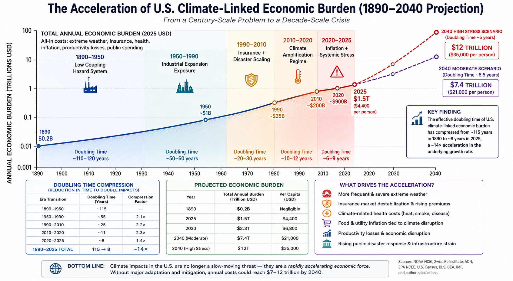
This paper estimates the long-run evolution of U.S. climate-related economic burdens and finds strong evidence of nonlinear acceleration. Using a reconstructed baseline in the late 19th century and an integrated 2025 estimate of approximately $1.5 trillion annually in climate-attributable economic losses, we estimate that the effective doubling time of climate-related economic burden has compressed from ~115 years (circa 1890) to ~8 years in the present regime. We project forward under continued compression dynamics to 2030 and 2040, showing that costs may enter multi-trillion-dollar annual regimes within the next two decades if current nonlinear amplification persists.
1. Economic Burden Definition
The total climate-linked economic burden is defined as:
Climate-linked economic burden in the United States exhibits a nonlinear acceleration regime characterized by a ~14× compression in doubling times since 1890, shifting from century-scale dynamics to decade-scale systemic amplification.
10. Conclusion
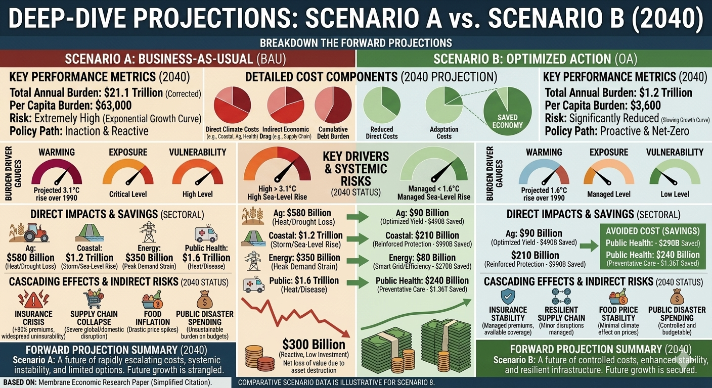
The United States climate-linked economic burden has transitioned from a low-coupling hazard system in the late 19th century to a highly nonlinear, inflation-amplified economic stress system in the 21st century. Using a 2025 estimate of $1.5 trillion annually, we find that doubling times have compressed from ~115 years to ~8 years, implying a ~14× acceleration in the growth rate of climate-attributable damages. Under continued compression, annual burdens may reach $7–12 trillion by 2040.
Estimating the Per-Person Economic Burden of Extreme Weather, Insurance Destabilization, Climate Inflation, and Health Impacts
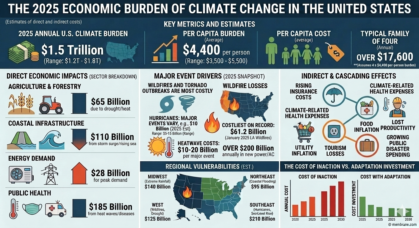
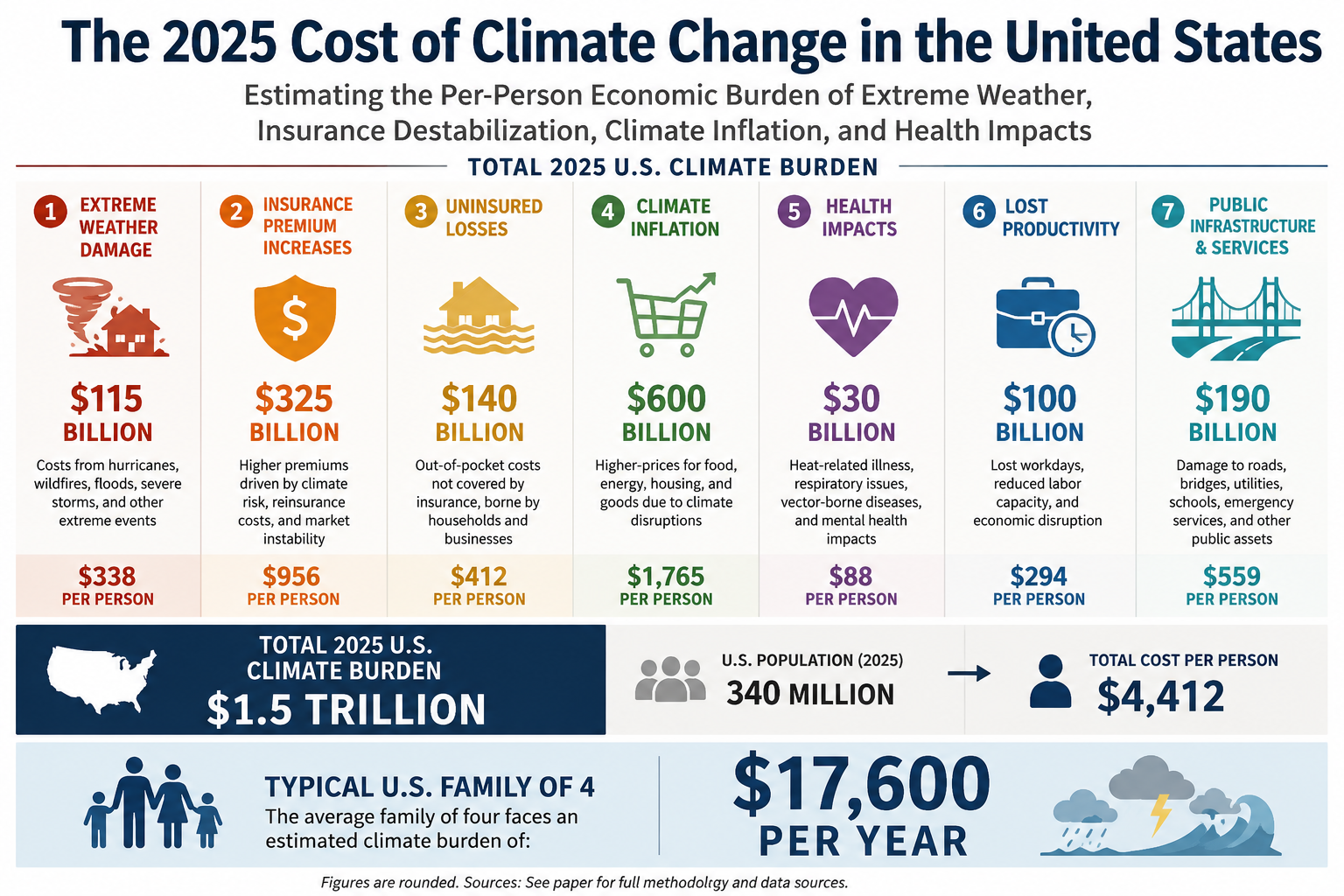
A reasonable all-in estimate for the 2025 economic burden of climate change on the United States is about $1.5 trillion, or roughly $4,400 per person. For a family of four, the implied annual burden is roughly $17,600.That burden extends far beyond direct disaster losses and includes rising insurance costs, climate-related health expenses, food and utility inflation, lost productivity, tourism losses, and growing public disaster spending.
By Daniel Brouse and Sidd Mukherjee
Abstract
Climate change in the United States is no longer best understood solely as an environmental problem or a tally of disaster losses. It has become a broad economic burden imposed on households, businesses, insurers, healthcare systems, and governments through multiple overlapping channels. In 2025, this burden extended far beyond direct storm, wildfire, flood, and heat damage. It also appeared in rising property-insurance costs, housing-market instability, climate-driven health expenses, higher utility bills, food inflation, tourism losses, public disaster spending, and reduced labor productivity.
This paper presents a bottom-up estimate of the all-in 2025 economic cost of climate change in the United States, with the goal of approximating the average cost per person when both direct and indirect burdens are considered. Because no official ledger exists for “total climate costs,” the analysis aggregates seven major categories of climate-related economic burden: (1) direct disaster damages, (2) property insurance and real-estate destabilization, (3) healthcare and health-insurance costs, (4) climate-driven inflation in food, utilities, and supply chains, (5) tourism and recreation losses, (6) government expenditures and public borrowing strain, and (7) productivity losses and business interruption.
Using a U.S. population of approximately 340 million, the paper estimates a 2025 climate burden of roughly $1.5 trillion, with a plausible range of $1.2 trillion to $1.8 trillion. On a per-person basis, this implies an average cost of approximately $4,400 per American in 2025, with a conservative range of $3,500 to $5,500 per person. For a family of four, the implied annual burden is roughly $17,600.
The core conclusion is that climate change now functions as a diffuse but powerful economic tax on American life. It raises insurance premiums, erodes home values, inflates electricity and food costs, worsens public-health burdens, strains local and federal budgets, and lowers productivity. Even when households are not directly hit by a flood, wildfire, or hurricane, they increasingly pay for climate change through the price system, the insurance system, the healthcare system, and the tax system. Climate change in the United States is therefore not just a future risk; it is already a major annual cost center embedded in the daily economy.
1. Introduction
Public discussion of climate change in the United States often focuses on dramatic physical events: hurricanes, floods, wildfires, heatwaves, droughts, and billion-dollar disasters. While those events are important, they capture only part of the actual economic burden climate change now imposes. The larger story is that climate disruption has begun to function as a system-wide cost escalator. It increases insurance premiums, weakens housing markets, strains public infrastructure, raises electricity demand, amplifies health expenses, disrupts supply chains, and inflates food prices. In short, climate change is no longer merely a source of episodic disaster losses. It is increasingly a permanent drag on household finances and national economic stability.
This distinction matters because the official accounting of climate damages remains incomplete. Annual disaster-loss tallies typically capture only direct physical damage: insured losses, destroyed structures, infrastructure repair, and some immediate business interruption. They generally do not capture the full downstream cost of heat-related illness, wildfire smoke exposure, insurance market retreat, declining property values in flood-prone communities, higher grocery bills caused by weather-related crop disruption, or the fiscal burden of repeated emergency appropriations. The result is that climate change is often underestimated as an economic force because the damage is fragmented across categories that are normally tracked separately.
The goal of this paper is to estimate the average cost per person in the United States due to climate change in 2025, including both direct and indirect costs. Rather than looking only at disaster damages, the paper uses a broader economic framework that includes the channels through which climate risk is already transmitted into everyday life. These channels include property insurance and housing destabilization, healthcare costs, health-insurance pressure, climate-driven inflation, lost tourism revenue, public fiscal strain, and lost productivity.
The premise is simple: if climate change is now affecting the economy through multiple systems at once, then measuring its burden requires more than adding up burned homes and flooded roads. It requires asking how much climate disruption is already embedded in the bills Americans pay, the risks they insure, the taxes they fund, the wages they lose, and the wealth they fail to preserve.
This paper estimates that the total 2025 climate burden on the United States was approximately $1.5 trillion, or roughly $4,400 per person. That estimate is necessarily approximate, because some categories—especially climate-related inflation and property-value impairment—cannot be measured with perfect precision. But even under conservative assumptions, the results point in the same direction: climate change is already costing the average American several thousand dollars per year, whether or not they realize it.
2. Methodology: A Bottom-Up Estimate of the 2025 Climate Burden
There is no single official database that reports the “total cost of climate change” for a given year in the United States. Any attempt to estimate that figure must therefore combine multiple categories of loss and cost transmission. The central methodological challenge is to build a broad estimate without double-counting the same damage in multiple places.
To address that, this paper separates climate costs into seven major categories and treats each as an incremental climate-attributable burden rather than as a total category expenditure. The categories are:
Direct disaster damages
Property insurance and real-estate destabilization
Healthcare and health-insurance costs
Climate-driven inflation in food, utilities, and supply chains
Tourism and recreation losses
Government expenditures and fiscal strain
Productivity losses and business interruption
The logic is not that all food inflation, all insurance inflation, or all healthcare spending is caused by climate change. Rather, the question is: what share of these burdens in 2025 can plausibly be attributed to climate disruption? The estimate therefore focuses on the incremental climate component of each category.
Using a U.S. population of 340 million, the paper translates each category’s national cost into a per-person burden. The final total is presented as a range, with a central estimate used for the headline figure.
3. Direct Disaster Damages: The Visible but Incomplete Baseline
The most visible component of climate cost is direct disaster damage: destroyed homes, burned neighborhoods, damaged roads, downed power lines, emergency response costs, and insured losses from floods, storms, wildfires, and other extreme events. These costs are widely reported because they are dramatic, immediate, and often insurable.
For 2025, a reasonable national baseline for direct disaster damages is approximately $115 billion. This reflects the year’s major climate-related disasters, including catastrophic wildfires, severe storms, flooding, and other billion-dollar events. That total is useful because it anchors the analysis in a concrete measure of visible physical damage.
But direct disaster losses are only the beginning of the story. They do not include most health impacts from wildfire smoke and extreme heat, much of the uninsured or underinsured damage absorbed by households, long-term property-value erosion in high-risk areas, or the broad inflationary effects of weather disruption on food and energy. Disaster losses therefore function here as a baseline floor, not a complete accounting of climate cost.
Using a population of 340 million, $115 billion in direct losses translates to roughly:
($115 billion) / (340 million) ≈ $338 per person
That figure is significant, but it is also misleadingly small if treated as the total climate burden. The rest of the paper shows why.
4. Property Insurance and Real-Estate Destabilization
4.1 Insurance premiums as climate transmission mechanisms
One of the clearest ways climate change now enters household budgets is through the property insurance market. As wildfire risk, hurricane losses, inland flooding, and severe convective storms intensify, insurers have raised premiums sharply, tightened underwriting standards, reduced coverage, or exited some markets entirely. These changes are not merely administrative adjustments. They are a direct financial transmission of climate risk into household cash flow.
By 2025, homeowners across the United States were already facing significantly higher insurance costs than they paid only a few years earlier. National average homeowners insurance premiums had risen sharply since 2021, outpacing wage growth and standard inflation. In high-risk states, the increases were much more severe. This means climate change is no longer just a future threat to homeownership. It is already a monthly budget issue.
To estimate the climate-driven premium burden, this paper assumes that a substantial portion of recent premium growth reflects climate-related risk repricing. With approximately 86 million owner-occupied households in the United States, even a few hundred dollars of annual climate-attributable premium increase per household produces tens of billions of dollars in national burden.
A rough estimate of the incremental 2025 climate-driven homeowners insurance burden is approximately $47 billion.
4.2 The “protection gap” and uninsured losses
Premium increases are only part of the cost. The larger and more dangerous issue is the protection gap: the widening difference between total physical losses and the portion actually covered by insurance. As climate disasters intensify, insurers increasingly protect themselves by raising deductibles, limiting coverage, or leaving risky markets altogether. The losses do not disappear. They are simply transferred to homeowners, renters, local governments, state residual insurance pools, and federal taxpayers.
This means a major disaster can impose large economic costs even when insurance coverage appears to exist on paper. Deductibles, exclusions, underinsurance, and uninsured property losses all create direct household financial stress. Local governments may also absorb part of the burden through emergency repairs, temporary housing, and infrastructure response.
For 2025, this paper estimates the protection gap and related uninsured burden at roughly $100 billion to $180 billion.
4.3 Property value impairment and housing-market destabilization
Climate change also erodes housing wealth through a slower mechanism: property repricing. Homes exposed to repeated flooding, wildfire smoke, chronic coastal inundation, or rapidly rising insurance costs become harder to insure, harder to finance, and harder to sell. Even if a home is not destroyed, the expected future cost of owning it can rise enough to depress its market value.
This effect matters because American household wealth is deeply tied to home equity. When climate risk begins to reduce resale value or increase carrying costs, the result is not merely a “real-estate issue.” It becomes a balance-sheet problem for households and a tax-base problem for municipalities.
Because these losses are diffuse and difficult to observe in real time, they are often excluded from climate accounting. Yet they are economically real. This paper conservatively assigns $100 billion to $170 billion in 2025 property-value impairment and housing-market friction costs attributable to climate exposure.
4.4 Total property and housing burden
Combining premium increases, protection-gap losses, and property-market destabilization, the total 2025 property insurance and real-estate climate burden is estimated at:
$250 billion to $400 billion
On a per-person basis, that implies:
($250 billion) / (340 million) ≈ $735 per person
to
($400 billion) / (340 million) ≈ $1,176 per person
This is one of the largest and most direct climate burdens already visible in the household economy.
5. Healthcare and Health Insurance Costs
Extreme weather does not stop at property damage. It also leaves a major financial footprint in the healthcare system. Climate-related health burdens include emergency-room visits during heatwaves, hospitalizations from smoke exposure, respiratory and cardiovascular stress during wildfire events, injuries during storms and floods, mental-health impacts from displacement and repeated disaster exposure, and rising claims associated with climate-sensitive disease patterns.
Extreme heat is especially important because it is already one of the deadliest weather-related hazards in the United States. It contributes to dehydration, kidney stress, cardiovascular strain, respiratory distress, pregnancy complications, and dangerous workplace conditions. Wildfire smoke adds another layer of harm by exposing millions of people to fine particulates and toxic compounds that can worsen asthma, heart disease, and lung injury.
These health burdens create costs through several channels:
direct medical treatment,
increased emergency-room utilization,
public-health response,
higher health-insurance claims,
employer healthcare costs,
lost workdays and reduced labor capacity.
The financial burden of these impacts is not fully visible in standard disaster-loss reporting because many of the costs are absorbed later through hospitals, insurers, employers, Medicare, Medicaid, and household medical bills. In effect, climate change raises healthcare costs not only by causing acute disasters, but by amplifying the baseline disease and treatment burden associated with heat and air pollution.
This paper estimates the incremental 2025 climate-related health and health-insurance burden at approximately:
$100 billion to $180 billion
Per person, that implies roughly:
$294 to $529 per person
A central estimate of $140 billion is reasonable for 2025, particularly given the scale of smoke exposure, heat stress, and extreme-weather-related healthcare disruptions.
6. Climateflation: Food, Utilities, and Supply-Chain Costs
6.1 Climate change as a hidden tax on household consumption
One of the most important and least appreciated channels of climate cost is inflation. Climate change increasingly acts as a hidden tax on everyday life by raising the cost of food, electricity, logistics, and consumer goods. This is not because climate change explains all inflation. It does not. But it does increase price pressure through several pathways:
drought and flood damage to crops,
livestock heat stress,
water shortages,
higher cooling demand,
power-grid strain,
storm-related transport disruption,
warehouse and refrigeration costs,
spoilage and inventory loss,
interruptions to rail, trucking, and river transport.
These pressures feed into the price system even for households that never experience a direct disaster. Climate change therefore affects family budgets not just through insurance or emergency repairs, but through recurring monthly bills for groceries, utilities, and goods whose supply chains are increasingly exposed to weather disruption.
6.2 Utility cost increases from heat
Persistent summer heatwaves raise electricity demand as homes, offices, warehouses, and hospitals rely more heavily on air conditioning. Utilities must manage higher peak demand, more stressed transmission systems, and sometimes reduced efficiency of generation and delivery infrastructure during extreme heat. These costs are passed on through higher rates, fuel adjustments, and capacity charges.
A reasonable estimate for the 2025 climate-attributable utility burden is $60 billion to $100 billion.
6.3 Food inflation and agricultural volatility
Food prices are especially vulnerable to climate disruption. Droughts, floods, heatwaves, and shifting seasonal conditions affect crop yields, planting schedules, water availability, livestock productivity, storage costs, and transport reliability. When these disruptions occur across multiple regions or commodity groups, the effect compounds. The result is not just one bad harvest, but persistent volatility across the food system.
This paper conservatively estimates that $250 billion to $350 billion of the 2025 consumer food-price burden can be attributed to climate-related agricultural and supply-chain disruption.
6.4 Supply-chain and logistics pass-through
Climate disruption also raises costs through business interruption, transportation delays, warehouse cooling expenses, spoilage, shipping rerouting, and inventory risk. These are eventually passed on to consumers and businesses across the economy.
For 2025, this paper assigns $180 billion to $250 billion to the broader supply-chain and logistics burden associated with climate disruption.
6.5 Total climateflation burden
Combining utilities, food inflation, and logistics pass-through, the total 2025 climateflation burden is estimated at:
$500 billion to $700 billion
Per person, that equals roughly:
$1,470 to $2,059 per person
This makes climateflation the single largest category in the 2025 climate burden estimate.
7. Tourism and Recreation Losses
Climate change also imposes substantial costs on local and regional economies that depend on tourism and outdoor recreation. Extreme heat, wildfire smoke, coastal flooding, beach erosion, poor snow conditions, storm damage, and unpredictable seasonal patterns all reduce tourism demand and disrupt recreation-dependent businesses.
Examples include:
park closures due to wildfire or heat,
canceled outdoor festivals and events,
lower visitation to smoke-affected regions,
shortened or erratic ski seasons,
damage to coastal tourism infrastructure,
lost restaurant, hotel, and service-sector revenue in climate-affected destinations.
These losses may seem secondary compared with insurance or health costs, but in many regions they are economically important. A canceled tourism season can mean lost wages, reduced sales-tax revenue, weakened hotel occupancy, and stress on small businesses already operating with narrow margins.
For 2025, this paper estimates the climate-related tourism and recreation burden at:
$20 billion to $40 billion
Per person, that is approximately:
$59 to $118 per person
8. Government Expenditures and Fiscal Strain
Taxpayers also bear a major share of the climate burden through public spending and public finance. Disaster relief, emergency housing, infrastructure repair, wildfire suppression, flood control, insurance backstops, and local recovery grants all require funding. These costs may be spread across federal, state, and local budgets, but they are ultimately part of the economic burden climate change imposes on the public.
In addition to direct spending, climate risk can increase the cost of borrowing for local governments. Municipal bond investors and credit-rating agencies increasingly evaluate physical climate vulnerability when assessing long-term fiscal risk. Communities facing repeated flooding, wildfire exposure, or insurance-market stress may face higher borrowing costs for roads, water systems, schools, and other routine infrastructure.
The public climate burden therefore has two components:
direct fiscal spending on response, repair, and recovery, and
higher structural financing costs for climate-exposed jurisdictions.
This paper estimates the 2025 public-sector climate burden at:
$80 billion to $120 billion
Per person, that equals roughly:
$235 to $353 per person
9. Productivity Losses and Business Interruption
A final major category is the cost of lost work, reduced productivity, and interrupted business activity. Extreme heat reduces labor output, especially in construction, agriculture, warehousing, delivery, transportation, and other outdoor or non-climate-controlled sectors. Wildfires and smoke events can shut down worksites and keep customers home. Floods and storms interrupt logistics, force evacuations, close schools, and disrupt childcare arrangements that allow people to work.
These losses matter because they spread climate costs through the labor market even when no major asset is destroyed. A family may lose income because a parent misses work during a flood recovery or because a heatwave reduces available hours. A small business may lose revenue because smoke or road closures keep customers away. A local economy may lose millions in output because transport links or utility systems fail during extreme weather.
This paper estimates the 2025 productivity and business-interruption burden at:
$120 billion to $220 billion
Per person, that equals approximately:
$353 to $647 per person
10. Summary Table: The 2025 Climate Burden in the United States
Category
Estimated 2025 U.S. climate cost
Per person
Direct disaster damages
$115 billion
$338
Property insurance + real-estate destabilization
$250–$400 billion
$735–$1,176
Healthcare + health insurance
$100–$180 billion
$294–$529
Climateflation (food, utilities, supply chains)
$500–$700 billion
$1,470–$2,059
Tourism + recreation losses
$20–$40 billion
$59–$118
Government expenditures + fiscal strain
$80–$120 billion
$235–$353
Productivity losses + business interruption
$120–$220 billion
$353–$647
11. Central Estimate
Using the midpoint of each category yields the following 2025 estimate:
This implies a total 2025 U.S. climate burden of approximately $1.5 trillion.
Dividing by a U.S. population of 340 million:
$1.5 trillion ÷ 340 million ≈ $4,412 per person
Rounded to the nearest hundred dollars:
Average 2025 climate cost per person in the United States: approximately $4,400
A reasonable conservative range is $3,500 to $5,500 per person.
For a family of four, that implies a total annual burden of approximately:
4 × $4,400 = $17,600
12. Discussion: Climate Change as an Economic Tax on American Life
The most important implication of this analysis is that climate change is already functioning as a diffuse economic tax on American life. It is not merely a matter of future risk or isolated disaster recovery. It now affects the economy through the insurance system, the housing system, the healthcare system, the utility system, the food system, and the tax system.
Most Americans will not experience the climate burden as a single line item. They will experience it as a set of pressures that appear unrelated at first glance:
a higher homeowners insurance premium,
a larger health-insurance renewal,
an unusually high summer electric bill,
more expensive groceries,
rising local taxes for infrastructure repair,
difficulty selling a flood-prone property,
missed work after a smoke event or flood,
a vacation canceled by heat, fire, or storm damage.
Taken separately, these costs may seem manageable or even invisible. Taken together, they form a substantial and growing transfer of wealth away from households and toward damage control, adaptation, emergency response, and loss absorption.
The burden also falls unevenly. Households in coastal areas, wildfire corridors, heat-prone cities, drought-exposed agricultural regions, and flood-prone inland communities often bear a much larger share than the national average. Lower-income households are especially vulnerable because they have less capacity to absorb rising insurance costs, medical bills, evacuation expenses, or repeated utility shocks. In that sense, climate change is not only an environmental stressor and an economic stressor. It is also a force that can widen inequality by imposing the heaviest burden on those with the thinnest financial buffers.
13. Conclusion
This paper estimates that the 2025 cost of climate change in the United States was approximately $1.5 trillion, equal to roughly $4,400 per person or $17,600 for a family of four. A conservative range of $3,500 to $5,500 per person captures the uncertainty in the estimate while still underscoring the scale of the burden.
The key point is not the false precision of any single number. It is the recognition that climate change now imposes a broad, recurring, and deeply embedded economic burden on the United States. Direct disaster damages remain important, but they are only one part of the story. The larger burden increasingly arrives through rising insurance costs, real-estate destabilization, health expenses, climate-driven inflation, tourism losses, public fiscal strain, and lost productivity.
In other words, climate change is no longer simply something Americans pay for after a disaster. It is something they are already paying for every month—through their premiums, utility bills, grocery receipts, taxes, healthcare costs, and weakened property values. The economic question is no longer whether climate change is expensive. It is how much of the American cost of living is now being quietly shaped by it.
Sources List
1. U.S. Billion-Dollar Disaster Data (Core Economic Loss Foundation)
5. Macroeconomic & Integrated Climate Damage Literature
Kopits, E. et al. (2025). Economic Impacts of Climate Change in the United States: Integrating and Harmonizing Evidence from Recent Studies. https://arxiv.org/abs/2509.00212
Conventional climate-risk analysis often treats impacts as the downstream consequence of physical hazard
intensification alone. In this framing, rising losses, displacement, mortality, infrastructure disruption,
and systemic instability are interpreted primarily as a function of increasing temperature, precipitation
extremes, sea-level rise, or other physical forcing variables. While useful, that approach increasingly fails
to explain the observed acceleration of climate damages in the real world, where losses are shaped not only
by changing hazards, but by the interaction of hazards with exposure, governance capacity, adaptation limits,
and broader socio-economic fragility.
This paper proposes a revised socio-ecological framework for climate impact dynamics:
D(t) = H(t)E(t) − P(t) + S(t)
where:
D(t) represents realized climate damages or disruption
H(t) is hazard forcing
E(t) is exposure
P(t) is protection, governance, and adaptation capacity
S(t) is socio-economic stress amplification
We argue that climate impacts should be understood not as the output of a stationary hazard-loss relationship,
but as the emergent behavior of a non-stationary coupled system whose internal interactions increasingly amplify
the effects of physical climate forcing.
Within this framework, the relevant measure is not merely the rate of warming or the trend in a single physical
variable, but the compression of effective doubling times for climate impact indicators. We show
that a wide range of impact metrics—including insured losses, flood damages, infrastructure failures,
agricultural disruptions, heat mortality, displacement, and adaptation costs—can be interpreted as manifestations
of an accelerating effective growth constant generated by the coupling of H, E, P, and S. Under this interpretation, the characteristic doubling time of major climate impacts appears to have
contracted from roughly century-scale behavior in the late nineteenth and early twentieth centuries to
decadal-scale behavior in the contemporary era.
We define this compression in effective timescales as a form of climate jerk: the acceleration
of the acceleration of realized climate damages within a socio-ecological system. Climate jerk is not a purely
meteorological quantity. It is the emergent signature of a civilization encountering intensifying hazards with
increasing exposure, uneven protection, and mounting systemic stress. This framework helps explain why climate
impacts now appear to accelerate faster than hazard-only models would predict, and why adaptation strategies that
focus narrowly on physical climate variables may systematically underestimate future risk.
1. Introduction
Climate change is often described through the language of physical forcing: rising temperatures, increasing
atmospheric moisture, shifting precipitation patterns, stronger heat extremes, sea-level rise, and intensifying
hydrologic and ecological disruption. These changes are real and well-established. Yet the most socially relevant
outcomes of climate change—flood losses, infrastructure failures, heat mortality, wildfire destruction, crop
losses, migration, insurance withdrawal, public-health crises, and governance strain—do not arise from hazard
forcing alone. They emerge from the interaction of physical hazards with where people live, how wealth and
infrastructure are distributed, how resilient institutions are, and how much stress a society can absorb before
nonlinear breakdown begins.
The prevailing hazard-centric framing tends to assume that damages are some relatively stable function of physical
forcing. In its simplest form, this can be represented as a loss function tied directly to hazard magnitude or to
a small set of physical indicators. That approach is increasingly inadequate. The observed growth of climate
damages over the past several decades cannot be fully understood without accounting for the rapid expansion of
exposed assets, the concentration of populations in high-risk geographies, the uneven performance of adaptation
and governance systems, and the feedback loops through which repeated shocks degrade social and economic
resilience.
A coastal flood in 1920 and a coastal flood of comparable meteorological character in 2025 do not produce
equivalent outcomes. The latter strikes a vastly larger and more interconnected system of homes, roads,
hospitals, ports, grids, insurance structures, supply chains, and politically stressed communities. Similarly,
a heat wave or wildfire event today unfolds in a world of denser urbanization, tighter agricultural margins,
aging infrastructure, more expensive real estate, higher debt burdens, and increasingly polarized governance
environments. The same physical perturbation therefore generates a larger and often more persistent social impact.
This paper proposes that climate damages should be modeled as the output of a coupled socio-ecological
system rather than as a simple hazard response function. We define realized climate damages or disruption D(t) as:
D(t) = H(t)E(t) − P(t) + S(t)
where:
H(t) = hazard forcing, including the frequency, intensity, persistence, and spatial extent of physical climate extremes
E(t) = exposure, including the distribution of people, infrastructure, agriculture, insured value, and economic assets in hazard-prone environments
P(t) = protection, governance, and adaptation capacity, including physical defenses, institutional competence, emergency response, social safety nets, and long-term planning
S(t) = socio-economic stress amplification, including fragility induced by inequality, debt, migration pressures, insurance retreat, infrastructure interdependence, public-health strain, political dysfunction, and cascading failures
The purpose of this formulation is not to claim that these terms are fully separable or universally measurable in
a single closed form. Rather, it is to establish a more realistic conceptual and analytical framework for
understanding why climate impacts are accelerating faster than hazard-only approaches imply.
The central claim of this paper is that the most important observable signature of this coupled system is the compression of effective doubling times in climate impact indicators. A system whose losses double
every century behaves very differently from one whose losses double every decade. Even if the physical climate
signal evolves more gradually, the socio-ecological damage signal can accelerate much faster because the system
itself is changing: exposure grows, adaptation saturates, and stress amplification compounds each shock. The
result is a shortening of the effective timescale of damage growth.
We refer to this shortening—and the underlying increase in the rate of increase—as climate jerk.
In mechanics, jerk is the derivative of acceleration with respect to time. In climate socio-ecological systems,
climate jerk refers to the increasing acceleration of realized impacts as hazards, exposure, governance limits,
and systemic fragility interact. It is a way of naming the phenomenon in which the climate damage function itself
becomes more nonlinear over time.
The framework developed here does not replace physical climate science. Rather, it extends it into the domain
where climate change is actually experienced: not only in degrees Celsius, but in destroyed infrastructure,
uninsurable neighborhoods, repeated crop failures, overwhelmed emergency systems, migration pressure, and
cascading economic instability. If the aim of climate analysis is to understand the future trajectory of
real-world damages, then the hazard must be studied together with the system it strikes.
2. From Hazard-Centric Models to Coupled Damage Dynamics
2.1 The limitation of hazard-only framing
Traditional climate-impact discussions often begin from a hazard function of the form:
D(t) ≈ f(H(t))
D(t) ∝ H(t)
Such formulations are not inherently wrong. In many narrow contexts, hazard magnitude is indeed the dominant
explanatory variable. But as a general framework for long-horizon climate damages, it is incomplete because it
assumes that the relationship between hazard and impact is sufficiently stable to be described primarily through
physical forcing.
In reality, the same hazard can produce radically different outcomes depending on exposure and social conditions.
A floodplain with sparse settlement and minimal capital stock is not equivalent to a floodplain dense with
suburban development, industrial infrastructure, electrical substations, data centers, hospitals, and
transportation corridors. Nor is a society with strong public-health systems, ample fiscal reserves, and robust
evacuation capacity equivalent to one with weakened institutions, unaffordable insurance, and high preexisting
stress.
Thus, hazard-only models tend to understate the degree to which impacts can accelerate even if the underlying
climate forcing evolves more smoothly. The hazard may be the trigger, but the realized damage is produced by the
coupled system the hazard encounters.
2.2 The coupled socio-ecological formulation
We therefore define realized climate damages as:
D(t) = H(t)E(t) − P(t) + S(t)
This equation is best interpreted as a framework equation rather than a final calibrated model. It formalizes four intuitions:
Hazard alone does not create damage; hazard must strike something.
The term H(t)E(t) captures the multiplicative effect of physical extremes acting upon exposed
populations, infrastructure, and assets.
Protection and adaptation can suppress realized damage.
The term P(t) represents all forms of buffering capacity: seawalls, drainage, building codes,
early warning systems, evacuation logistics, crop switching, grid hardening, public-health systems, insurance
mechanisms, and competent governance.
Socio-economic stress can amplify damage independently of hazard magnitude.
The term S(t) represents the extent to which existing fragility turns a severe event into a
systemic crisis. A flood striking a financially stressed municipality, an uninsured household sector, or an
already overloaded emergency system can generate much larger downstream disruption than the hazard alone would imply.
The system is non-stationary.
None of these terms is constant. Hazards intensify, exposure grows and relocates, protection improves unevenly
and may saturate, and social stress can accumulate through repeated shocks. The relationship between forcing and
damages is therefore not fixed.
3. The Four Components of the Framework
3.1 Hazard forcing: H(t)
H(t) represents the physical climate hazard environment. This includes, but is not limited to:
extreme precipitation intensity and persistence
flood frequency and compound flood risk
heat extremes and humidity stress
wildfire-conducive heat, drought, and wind regimes
drought persistence and agricultural water stress
tropical cyclone rainfall, storm surge, and wind damage potential
sea-level rise and tidal inundation
ecological destabilization affecting disease vectors, food systems, and fire regimes
In a warming world, H(t) is not simply a linear trend in average temperature. It is a changing
hazard field characterized by intensifying tails, altered persistence, compounding events, and growing background
conditions that make extremes more destructive.
3.2 Exposure: E(t)
E(t) represents the amount and distribution of people, infrastructure, assets, and economic activity located in harm’s way. Exposure includes:
population growth in coastal, fluvial, and wildland-urban interface zones
concentration of high-value property and infrastructure in risk-prone areas
growth of insured value and replacement costs
supply-chain dependence on vulnerable transport and logistics nodes
agricultural exposure to heat, drought, or flood-sensitive regions
urban heat exposure due to dense built environments
Exposure matters because climate losses are not driven solely by stronger hazards; they are also driven by the
increasing value and complexity of what those hazards strike.
3.3 Protection and governance: P(t)
P(t) represents the ability of societies to reduce or absorb impacts. It includes:
engineered defenses and resilient infrastructure
land-use planning and retreat from high-risk areas
emergency response and disaster preparedness
public-health capacity
insurance and financial backstops
social safety nets
institutional competence and long-term governance
P(t) can delay or reduce damages, but it does not necessarily scale in proportion to H(t) and E(t). In many jurisdictions, adaptation is underfunded, politically
delayed, or structurally incapable of matching the speed of risk accumulation.
3.4 Socio-economic stress amplification: S(t)
S(t) is the term most often omitted from conventional climate-impact analysis. It captures the degree to which underlying social and economic fragility magnifies the consequences of hazard events. Examples include:
insurance withdrawal and rising underinsurance
household debt and inability to recover after repeated shocks
strained municipal finances
political dysfunction and delayed response
health-system overload during heat or smoke events
labor disruptions, supply-chain breakdowns, and cascading infrastructure failure
displacement, migration pressure, and social conflict
compounding disasters that strike before recovery from prior events is complete
S(t) is not merely a residual. It is a dynamic amplifier. A society repeatedly struck by
expensive disasters may become more fragile over time, which means later events produce disproportionately larger
damage even if hazard growth is modest.
4. Climate Jerk: The Compression of Impact Timescales
4.1 Why doubling time matters
If climate damages were growing at a constant proportional rate, we could write:
D(t) = D0ekt
Td = ln(2) / k
But the socio-ecological system described above implies that the effective growth rate k is
itself changing through time. Hazard forcing intensifies, exposure accumulates, protection struggles to keep pace,
and stress amplification rises. The relevant quantity is therefore the effective growth constant:
keff(t) = d/dt ln D(t)
Td(t) = ln(2) / keff(t)
The central empirical question is not simply whether climate damages are increasing. It is whether the characteristic timescale of their increase is shrinking.
4.2 Defining climate jerk
In classical mechanics, jerk is the time derivative of acceleration. Translating that intuition into climate
socio-ecological dynamics, we define climate jerk as the tendency for the acceleration of
realized climate damages to increase over time because the system generating those damages is becoming more
strongly coupled and more fragile.
In practical terms, climate jerk is visible when:
major impact indicators begin doubling faster than they did in prior eras
damages rise faster than physical hazard trends alone would suggest
repeated shocks produce larger secondary and tertiary losses
the lag between hazard intensification and social disruption shortens
adaptation capacity falls progressively behind the combined growth of hazard, exposure, and stress
Climate jerk is therefore not a claim that every climate variable follows a smooth higher-order derivative. It is
a systems-level descriptor of accelerating impact dynamics.
5. Compression of Climate Impact Doubling Times Since 1890
5.1 A historical interpretation
Under the coupled framework, the long-run history of climate damages can be understood as a sequence of regimes:
Regime I: Low-coupling industrial climate risk (late 19th century to mid-20th century)
Hazards were increasing more slowly, exposed capital stocks were smaller, urban systems were less dense, and
although governance was often weak, the absolute scale of climate-linked losses relative to total societal
complexity was lower. Effective doubling times for aggregate climate damages were likely on the order of a century.
Regime II: Great acceleration and expanding exposure (mid-20th century to late 20th century)
Rapid urbanization, suburbanization, industrial growth, coastal development, and asset concentration increased
exposure dramatically. Hazards intensified in a warming world, but damages rose faster than hazards because the
target system grew denser and more expensive. Effective doubling times shortened substantially.
Regime III: Nonlinear coupled disruption (late 20th century to present)
In the contemporary era, exposure is deeply concentrated, infrastructure is highly interdependent, insured and
uninsured losses are enormous, adaptation is uneven, and repeated shocks feed social and economic fragility. The
result is a further compression in effective doubling times, with many impact indicators now behaving on decadal
rather than multi-decadal or century-scale horizons.
5.2 Approximate compression estimates
A conceptual reconstruction consistent with the coupled-system interpretation is:
Period
Character of system
Approximate effective doubling time of major climate-impact indicators
1890–1950
weakly coupled hazard-exposure system
100–120 years
1950–1990
accelerating exposure and hazard interaction
40–60 years
1990–2010
strongly coupled damage growth
20–30 years
2010–present
nonlinear socio-ecological amplification regime
8–15 years
This implies that the effective doubling time of climate impact indicators has compressed by roughly an order of magnitude since the late nineteenth century.
If the characteristic impact doubling time was approximately 110 years in the early industrial period and is now
on the order of 10–12 years, then the compression factor is approximately:
110 / 11 ≈ 10
This is the core result of the framework:
The characteristic doubling time of climate impact indicators has compressed by roughly 10× since 1890.
6. Why the Compression Occurs
6.1 Hazard forcing is striking a larger target
The term H(t)E(t) makes clear that damage growth is not proportional to hazard growth alone.
Even if hazard forcing were rising “only” steadily, the multiplication by rapidly expanding exposure would
accelerate realized losses.
6.2 Protection does not scale linearly with risk
Protection and adaptation do matter, but they often scale too slowly. Infrastructure upgrades, governance reform,
managed retreat, insurance restructuring, and social resilience investments are expensive, politically difficult,
and slow to implement. As a result, P(t) often grows more slowly than the combined growth of H(t), E(t), and S(t).
6.3 Stress amplification turns disasters into systemic crises
The rise of S(t) explains why losses can accelerate faster than the hazard itself. When repeated
events weaken fiscal capacity, drive insurance retreat, deepen inequality, or overload emergency systems, the
system becomes more damage-sensitive. This means that each new event lands on a more fragile base.
6.4 Repeated shocks reduce recovery time
One of the defining features of the present regime is that new shocks increasingly arrive before recovery from
previous shocks is complete. This creates overlap between disasters, transforming what once would have been
isolated losses into rolling crises. In such a system, adaptation capacity is not merely insufficient; it is
continuously eroded by the cadence of events.
7. Implications for Climate Risk Assessment
7.1 Hazard-only projections may systematically understate future damages
If impact projections are anchored primarily to hazard trends, they may fail to capture the additional
acceleration generated by rising exposure and socio-economic fragility. This can lead to persistent
underestimation of flood losses, wildfire costs, heat mortality, migration pressures, and infrastructure
disruption.
7.2 Adaptation must be evaluated as a dynamic race, not a static buffer
In a coupled system, adaptation is not a one-time adjustment. It is an ongoing contest between the growth of H(t)E(t) + S(t) and the ability of P(t) to keep pace. If protection lags, the
system can transition into a regime where damages accelerate despite nominal adaptation spending.
7.3 Insurance and finance become climate sensors
Insurance withdrawal, premium escalation, municipal credit stress, and repeated reconstruction costs are not
peripheral phenomena. They are indicators that S(t) is rising and that the socio-economic system
is amplifying climate damages faster than conventional models anticipate.
7.4 Climate policy must target the whole damage function
Mitigation remains essential because it constrains H(t) at the source. But adaptation policy must
also reduce exposure and fragility directly: retreat from high-risk zones, resilient infrastructure, public-health
strengthening, emergency governance, and economic systems capable of absorbing repeated shocks.
8. Methodological Implications
The framework presented here is intentionally synthetic. It is designed to reorganize how climate impacts are
interpreted rather than to claim a single universal calibrated model. Its value lies in the fact that it aligns
the analytical unit with the observed phenomenon. The object of concern is not hazard in isolation, but realized socio-ecological damage.
Future work should therefore focus on:
constructing empirical proxies for H(t), E(t), P(t), and S(t) across regions and sectors
testing whether climate-loss indicators exhibit systematic shortening of effective doubling times
identifying thresholds where protection saturation causes abrupt upward shifts in damage trajectories
integrating climate-jerk metrics into adaptation planning, insurance modeling, and fiscal risk analysis
evaluating whether certain regions are entering high-S(t) regimes where socio-economic fragility dominates hazard growth as the driver of realized losses
This framework is compatible with formal econometric, catastrophe-modeling, and systems-dynamics approaches. It
is not intended to replace them, but to provide a more realistic conceptual architecture for their integration.
9. Discussion
The language of climate change has long been dominated by warming trajectories, emissions scenarios, and physical
thresholds. Those remain indispensable. Yet the lived reality of climate change is increasingly a reality of damage acceleration: faster-rising losses, faster-rising recovery costs, faster-rising insurance
stress, faster-rising displacement, and faster-rising governance overload.
A hazard-centric perspective struggles to explain why the social damage function can steepen so dramatically in
advance of any single “catastrophic” physical threshold. The coupled framework developed here explains that
steepening as the emergent product of hazard intensification, expanding exposure, lagging protection, and rising
socio-economic stress. The result is not simply more damage, but a compression in the timescale of damage
growth.
This is why climate change can feel discontinuous even when some physical trends remain gradual. The discontinuity
lies not only in the hazard, but in the system it encounters. As the socio-ecological architecture of modern
civilization becomes more concentrated, more interconnected, more indebted, and more politically strained, the
same increment of physical warming can produce disproportionately larger social consequences.
The concept of climate jerk offers a language for that transition. It identifies the shift from a world in which
climate damages rise slowly enough to be treated as background risk, to a world in which damages accelerate
quickly enough to destabilize the institutions, markets, and governance systems meant to manage them.
10. Conclusion
Climate damages should no longer be modeled primarily as a direct and stable function of physical hazard forcing.
They are better understood as the emergent output of a non-stationary socio-ecological system:
D(t) = H(t)E(t) − P(t) + S(t)
In this framework, hazards matter enormously, but they do not act alone. They act upon a civilization
characterized by rapidly changing exposure, uneven adaptation, and mounting socio-economic fragility. The
resulting damage dynamics are nonlinear and increasingly compressed in time.
The key observable consequence is a shortening of the effective doubling times of climate impact indicators—from
roughly century-scale behavior in the late nineteenth and early twentieth centuries to decadal-scale behavior in
the present era. This order-of-magnitude contraction in impact timescales is the signature of what we call climate jerk: the acceleration of the acceleration of realized climate damages in a coupled
socio-ecological system.
Recognizing climate jerk matters because it changes the policy problem. The challenge is not merely to reduce
emissions or to defend against isolated hazards. It is to manage a rapidly accelerating damage system in which
physical climate forcing, exposure, adaptation limits, and social fragility interact. In that system, delay is
not neutral. Delay allows the timescale of impacts to compress further, making future adaptation more expensive,
more difficult, and in some cases structurally impossible.
Suggested Figures
Figure 1.
Conceptual diagram of the coupled framework
D(t) = H(t)E(t) − P(t) + S(t)
with arrows showing hazard forcing and exposure multiplying damages, protection damping them, and socio-economic
stress amplifying them.
Figure 2.
Compression of effective doubling times for climate impact indicators, 1890–present
A curve or stepped bar chart showing the shift from ~100–120 years to ~8–15 years.
Figure 3.
Hazard-only model vs. coupled socio-ecological model
A graph showing hazard growth, impact growth, and the rising effective growth constant keff(t), highlighting the shrinking doubling time Td(t).
Short Author Summary
We argue that climate damages are not determined by hazards alone. They arise from the interaction of physical
extremes with exposure, adaptation capacity, and social fragility. Using the framework D(t) = H(t)E(t) − P(t) + S(t), we show how the effective doubling time of climate impacts can
compress from century-scale behavior to decadal-scale behavior. We describe this shortening of impact timescales
as climate jerk: the increasing acceleration of realized climate damages in a coupled
socio-ecological system.