☁️🌎 LOW-LEVEL CLOUD FEEDBACK: THE UNKNOWN MEGA-MULTIPLIER
What if one of Earth’s most important climate amplifiers is something we still don’t fully understand?
Low-level marine clouds are more than weather. They are a planetary sunshade—reflecting enormous amounts of incoming sunlight back into space.
But what happens if that sunshade starts to disappear?
🔥 As the climate warms, low-level clouds over the Pacific may thin, weaken, and potentially reach a tipping point where marine stratocumulus cloud decks fragment.
Less reflective cloud cover means more sunlight reaches the dark ocean.
More absorbed solar energy means more warming.
And more warming can further disrupt the clouds.
That is a feedback loop.
But the bigger concern is what happens when this feedback couples with other warming feedbacks already accelerating across the Earth system.
🌀 Warming ↓ ☁️ Low clouds diminish ↓ ☀️ More solar energy enters the ocean ↓ 🌊 Ocean warming accelerates ↓ 🔥 Further climate warming ↓ ☁️ More cloud disruption
Leading research suggests that the loss of low-level cloud albedo could contribute an additional 1.5°C to 2°C of global warming.
That would not be a minor correction to the climate trajectory.
It may be The Mega-Multiplier. In a tipping point scenario where clouds completely break up under extreme emission tracks, it could trigger a catastrophic, abrupt warming spike.
The climate system is not a collection of isolated feedbacks.
It is a coupled, nonlinear system in which feedbacks can interact, reinforce one another, and accelerate change.
☁️ The clouds may be one of the biggest unknowns.
And the Pacific may be where we need to look.
Read the full paper and explore the feedback cascade:
The Mega-Multiplier
The dynamic role of clouds is widely recognized as the single largest source of uncertainty in modern climate modeling. Cloud feedbacks can act as both blankets, trapping Earth’s heat, and sunshades, reflecting sunlight back into space.
As global warming has entered a faster decadal phase, leading research indicates that changes to both high- and low-level cloud structures are shifting toward a strong, positive warming-amplification loop.
1. High-Level Clouds: The Expanding Heat Trap
High-level clouds, such as cirrus clouds, reside above 20,000 feet. Composed primarily of ice crystals, they are relatively thin and transparent to incoming solar radiation, allowing sunlight to pass through them. However, they are highly effective at absorbing the outgoing longwave infrared radiation—heat—emitted from Earth’s surface and re-radiating it back downward.
The Anvil Cloud Expansion: Deep convective storms in the tropics create massive, fan-shaped high clouds known as tropical anvil clouds. As the upper troposphere warms and shifts, these clouds are expected to remain at higher, colder altitudes. Because they are colder, they radiate less heat out to space, increasing their efficiency as a planetary heat trap.
The High-Cloud Shift: Furthermore, climate models suggest that warming causes high-level clouds to shift toward higher latitudes, or poleward. This migration redistributes the heat-trapping effect over areas that are already experiencing accelerated melting, like the Arctic, compounding regional warming trends.
2. Low-Level Clouds: The Diminishing Planetary Sunshade
While high clouds act as greenhouse blankets, low-level clouds—specifically marine stratocumulus decks that sit below 6,000 feet—act as Earth’s primary solar sunshade. They cover roughly 20% of the subtropical oceans and reflect up to 30% to 60% of incoming sunlight back into space.
The shrinking of these low-level cloud decks, particularly over the northeast and southeast Pacific Ocean, is the focal point of intense scientific concern.
The Mechanics of Pacific Cloud Loss
Low-lying marine stratocumulus clouds depend heavily on a fragile thermal balance. They are sustained by a process called cloud-top radiative cooling, in which the tops of the clouds radiate heat out into space, cooling the air within the cloud layer. This cooling causes the air to sink, creating a convective loop that draws moisture up from the warm ocean surface below to maintain the cloud deck.
Global warming disrupts this system in two powerful ways:
Atmospheric Opacity: High concentrations of greenhouse gases render the lower atmosphere more opaque to infrared radiation. This traps heat above the clouds, warming their tops and stifling the cloud-top radiative cooling required to drive convection.
Enhanced Evaporation and Turbulence: As sea-surface temperature (SST) rises, the layer of dry air above the marine boundary layer grows warmer. This induces stronger turbulence that entrains—pulls down—dry, warm air from above, rapidly evaporating the thin cloud layer.
Groundbreaking thermodynamic simulations, notably led by researchers at Caltech’s Linde Center, have revealed that low-level clouds possess a critical tipping point.
If greenhouse gas concentrations continue to rise unchecked, marine stratocumulus decks over the Pacific could reach an instability threshold where they fragment and dissolve into scattered, shallow cumulus clouds. Without the vast reflective white sheets to shield the ocean, the dark tropical and subtropical waters would absorb massive amounts of solar energy.
Calculations indicate that the loss of this cloud albedo feedback alone could add an additional 1.5°C to 2°C of global warming. In a tipping point scenario where clouds completely break up under extreme emission tracks, it could trigger a catastrophic, abrupt warming spike.
Even short of a total breakup, observational data from satellites indicates that a gradual thinning of these clouds is already underway. This slow degradation is believed to be a major factor behind the recent acceleration in Earth’s total energy imbalance and ocean heat uptake.
The Unknown Mega-Multiplier
Cloud feedback is different from many other climate feedbacks because the direction, magnitude, and interactions of cloud changes remain exceptionally difficult to constrain.
The fundamental physics are clear: clouds can either reflect incoming solar energy back into space or trap outgoing heat within the climate system. But their response to a warming planet depends on where clouds form, how high they are, how thick they become, how long they persist, how they interact with atmospheric moisture and circulation, and how those changes couple with other climate feedbacks.
That creates the possibility of a multiplier effect.
A reduction in low-level Pacific clouds allows more solar energy to enter the ocean. Additional ocean warming changes evaporation, atmospheric circulation, and moisture transport. Those changes can alter cloud formation and persistence, potentially producing further reductions in reflective cloud cover. At the same time, changes in high-level clouds can increase the retention of outgoing heat.
The result is not simply more warming.
It is a potentially coupled feedback cascade:
Warming → cloud changes → altered albedo and heat retention → more absorbed energy → additional warming → further cloud changes.
This is why low-level cloud feedback may represent one of the most consequential uncertainties in the future climate trajectory.
If Pacific low-level cloud cover continues to diminish, the planet loses part of its natural solar shield at precisely the time that greenhouse-gas concentrations are increasing and other climate feedbacks are accelerating.
The question is no longer simply whether clouds respond to warming.
The critical question is whether warming is pushing the cloud system toward a threshold where the loss of low-level marine cloud albedo becomes a self-reinforcing source of additional global warming.
If so, low-level cloud feedback could become the unknown mega-multiplier—a climate feedback capable of coupling with other tipping elements and accelerating an already nonlinear Earth-system response.
Climate feedbacks are processes in which an initial change in Earth’s climate system triggers additional changes that amplify or dampen the original change. Positive feedbacks amplify the initial warming caused by greenhouse-gas emissions, accelerating climate change beyond what the initial forcing alone would produce.
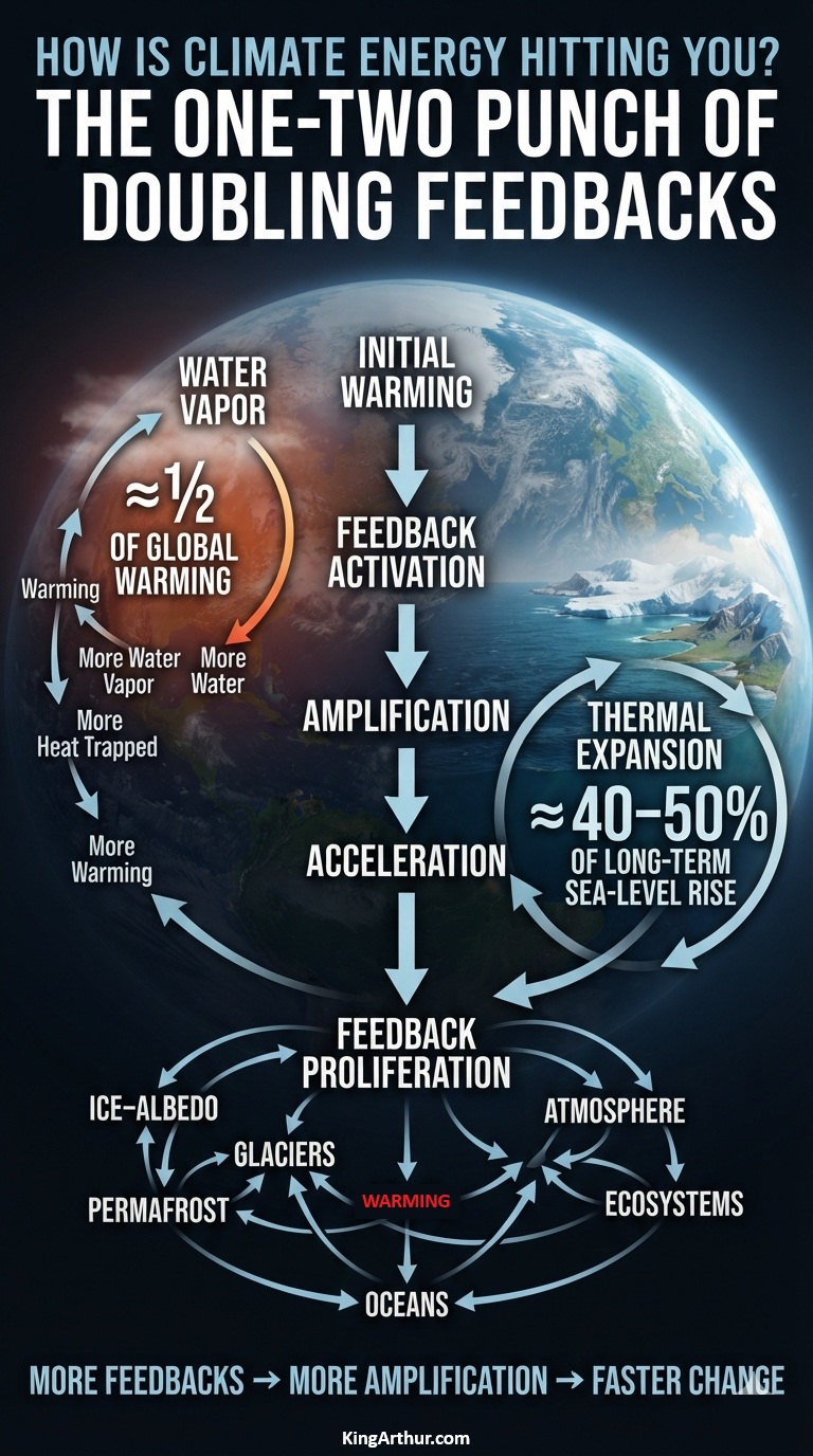
As Earth’s climate system warms and destabilizes, millions of emerging feedback interactions are becoming active across the atmosphere, oceans, cryosphere, land, and living systems. Many of these interactions are now being observed for the first time in human history. As individual feedbacks activate, strengthen, and interact with one another, they create new pathways for amplifying climate change and accelerating Earth-system change.
Two important climate-system responses illustrate this one-two punch: water-vapor amplification and ocean thermal expansion.
Water Vapor: The First Punch
Water vapor is Earth’s most important natural greenhouse-gas feedback.
As the atmosphere warms, it can hold more water vapor. Because water vapor is itself a powerful greenhouse gas, additional atmospheric moisture traps more outgoing infrared radiation, causing further warming. That additional warming allows the atmosphere to hold still more water vapor.
It is a reinforcing cycle:
Warming → more water vapor → more heat trapped → more warming
Water-vapor feedback is Earth’s greatest climate amplifier. As temperatures rise, the atmosphere holds more water vapor, which traps additional heat and amplifies the initial warming. Water-vapor feedback is responsible for approximately half of the global warming observed since the 1990s, making it one of the most powerful mechanisms accelerating Earth-system warming.
Thermal Expansion: The Second Punch
The ocean delivers a different kind of climate response.
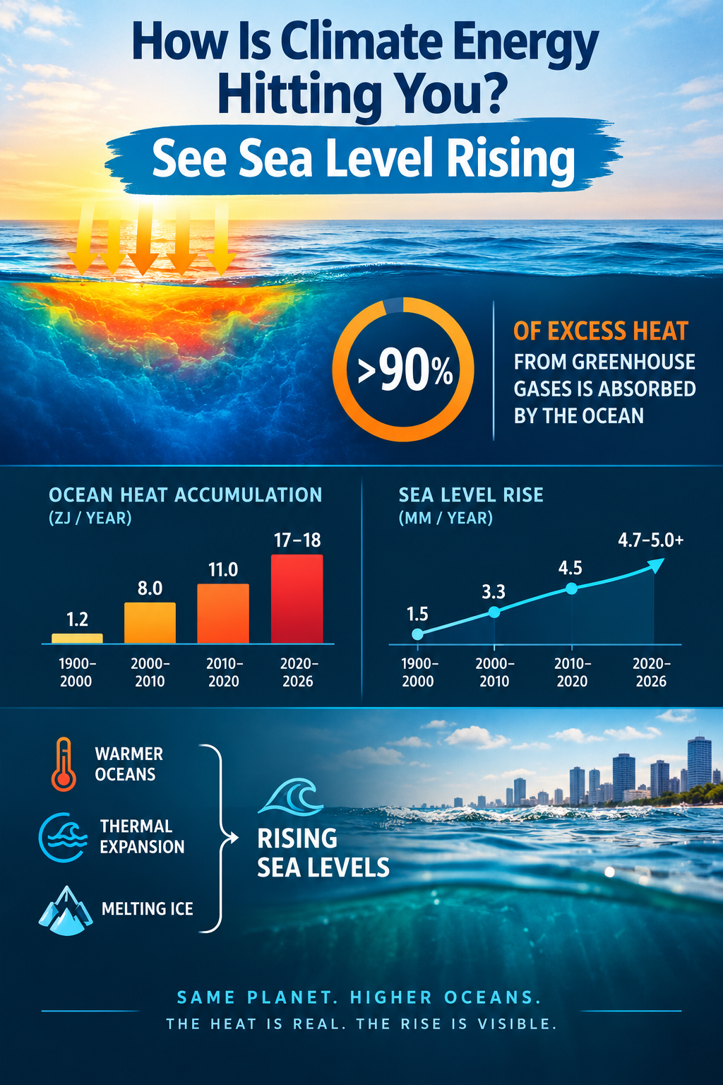
More than 90% of the excess heat accumulating in the Earth system is absorbed by the ocean. As seawater warms, it expands, increasing ocean volume and contributing to global sea-level rise.
This process is called thermal expansion or steric sea-level rise.
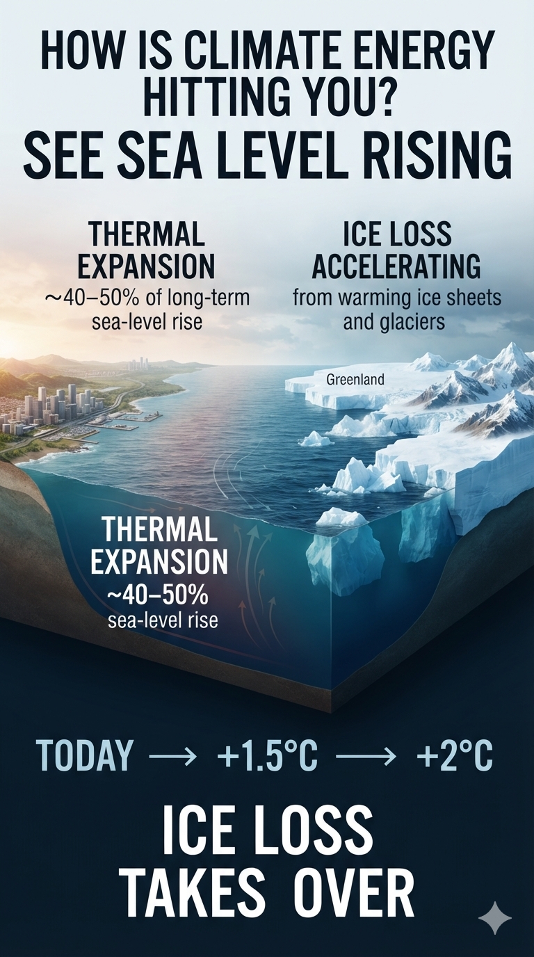
Thermal expansion has historically contributed roughly 40% to 50% of long-term global sea-level rise, with the remainder coming primarily from melting glaciers and ice sheets. The exact contribution varies over time and depends on the period and measurement method.
The water-vapor and thermal-expansion processes demonstrate two different ways excess climate energy can double the impact of climate change. Water-vapor feedback can approximately double the warming impact of greenhouse-gas emissions, while thermal expansion can approximately double the sea-level-rise impact by adding substantial additional sea-level rise beyond the contribution from melting land ice alone.
Water vapor amplifies warming.
Thermal expansion raises the oceans.
And neither operates in isolation.
As warming increases, additional feedbacks can become activated or strengthened—including ice-albedo feedback, permafrost carbon release, glacier and ice-sheet loss, and changes in ocean and atmospheric circulation.
The result is not a simple linear response.
More warming → more feedbacks → more warming → greater physical impacts
That is the one-two punch of climate feedbacks: the initial energy imbalance changes the climate system, while reinforcing processes can amplify the consequences.
The question is no longer simply “How much has Earth warmed?”
The more consequential question is:
“What is that additional climate energy doing to the Earth system—and how quickly are the feedbacks making it worse?”
More than 90% of the excess heat trapped in Earth’s climate system by human-caused greenhouse gas emissions is absorbed by the ocean.
Because water has a much higher heat capacity than air, the global ocean acts as a massive climate buffer. Without this vast heat reservoir soaking up the energy from burning fossil fuels, the atmosphere and land surfaces would be warming at a drastically faster, potentially unlivable rate.
But the ocean’s ability to absorb heat does not make that energy disappear. It stores the energy and redistributes it throughout the climate system—with consequences that include rising sea levels, melting ice, changing ocean circulation, and increasingly energetic climate feedbacks.
Estimated Rates of Ocean Heat Accumulation
Period
Approximate Rate
1900–2000
~1.2 ZJ/year
2000–2010
~8.0 ZJ/year
2010–2020
~11.0 ZJ/year
2020–2026
~17.0–18.0 ZJ/year
Key Factors Behind the 2026 Update
The 2025–2026 Acceleration
The 2020–2025 baseline average of approximately 16 ZJ/year was shattered by a massive, record-breaking surge reported in early 2026.
Peer-reviewed findings from the Institute of Atmospheric Physics (IAP/CAS) and Copernicus Marine revealed that the ocean absorbed an astonishing ~23 ZJ of excess heat in 2025 alone—up from ~16 ZJ in 2024.
That increase represents more than simply a large amount of additional heat. It is evidence of an accelerating rate of energy accumulation in the ocean.
Thermal Expansion
Thermal expansion is responsible for roughly 40% to 50% of long-term global sea-level rise. Over the last few decades, the drivers of rising oceans have generally been split roughly down the middle between thermal expansion—the swelling of water as it heats up—and meltwater from glaciers and ice sheets.
The percentage can fluctuate dramatically from year to year because of global weather patterns.
For instance, according to a NASA analysis, a massive surge in ocean heat during the 2024 El Niño caused a temporary flip: two-thirds, or about 66%, of that year’s accelerated sea-level rise came from thermal expansion alone.
Because the ocean is so vast, it acts like a giant, slow-moving thermal battery. Even if global greenhouse gas emissions were to completely stop today, the heat already trapped in the climate system would continue to move into the deep ocean for centuries.
This means sea levels will continue to rise from thermal expansion long after surface temperatures stabilize. As global temperatures rise beyond 1.5°C to 2°C, the rate of ice sheet melt is projected to grow exponentially, drastically outpacing thermal expansion. By the end of the century, scientists expect melting ice sheets and glaciers to become the overwhelmingly dominant driver, shrinking thermal expansion’s proportional share well below its current 40%–50% baseline.
The ocean therefore provides a critical buffer against even faster atmospheric warming—but that buffer comes with a cost. The energy being absorbed by the ocean is physically expanding the water and helping drive sea-level rise.
Rate of Sea-Level Rise
Period
Approximate Rate
1900–2000
~1.5 mm/year
2000–2010
~3.3 mm/year
2010–2020
~4.5 mm/year
2020–2026
~4.7–5.0+ mm/year
Sea Level Rise Is Accelerating
Sea-level rise is not occurring at a constant rate.
The rate has increased substantially over the past century, from roughly 1.5 mm/year during 1900–2000 to approximately 4.7–5.0+ mm/year during 2020–2026.
In other words, sea level rise is accelerating—and the acceleration itself is accelerating.
What happens in the ocean does not stay in the ocean.
The heat accumulating in the world’s oceans is becoming a physical signal we can see: sea level rising.
Reservoir Dry Dogs: Climate Change Is Shrinking America’s Water Storage
Climate change is making the world’s reservoirs less reliable, altering both the quantity and quality of stored freshwater. Rising temperatures, erratic precipitation, drought, wildfire, extreme rainfall, and shifting ecosystems are attacking water storage through three interconnected mechanisms:
Less water entering reservoirs
Less capacity to store the water that does arrive
Degrading water quality and creating additional climate feedbacks
The result is a growing climate-water squeeze: the water supply is declining while the infrastructure designed to store that water is simultaneously losing capacity.
The Global Reservoir Problem
More than half of the world’s largest reservoirs and lakes have shrunk significantly since the early 1990s as a result of climate change, extreme drought, human water consumption, and rapid sedimentation.
Research published in journals including Science and Nature Sustainability indicates that nearly two-thirds of existing large reservoirs have experienced substantial water losses.
This is not simply a drought problem. It is increasingly a water-storage problem.
The Colorado River System
Lake Mead and Lake Powell are the two largest reservoirs in the United States, supplied by the Colorado River system.
A multi-decade, climate-change-driven megadrought combined with heavy regional water demand has pushed both reservoirs toward historically low levels. Persistent low storage threatens drinking-water supplies and hydropower generation serving more than 40 million people across the American Southwest.
Frequently near-empty; severe farm-supply deficits
Strontia Springs
Colorado
Denver municipal supply
Wildfire erosion & flash floods
Rapid sediment buildup and declining storage capacity
San Luis
California / Central Valley
Agricultural & municipal hub
Atmospheric rivers & extreme heat
High runoff pollution, increasing groundwater dependence
Global Climate-Water Hotspots
The most critically impacted reservoirs and water systems around the world are experiencing intense climate-related strain.
Reservoir / Lake
Location
Primary Climate Driver
Status / Impact
Lake Mead & Lake Powell
United States
Megadrought & low snowmelt
Drinking-water and energy deficits
Balbina Reservoir
Brazil
High heat & decaying biomass
Massive methane emissions and ecological damage
Gowd-e-Zareh
Afghanistan
Extreme heat & runoff loss
Widespread desiccation and loss of agricultural water
Mar Chiquita
Argentina
Accelerated evaporation & land pressure
Severe shrinkage and ecological threat
These examples illustrate an increasingly important principle: climate change does not have to eliminate a water source completely to make the water system fail.
Extreme Evaporation
One of the simplest ways climate energy attacks reservoirs is through evaporation.
For an open water surface—including a reservoir or swimming pool—evaporation depends on several interacting variables. A useful framework is the Penman combination equation, which incorporates both the energy available at the surface and aerodynamic drying.
The equation contains two major physical components.
1. Available Energy
The term:
Δ(Rₙ − G)
represents the energy available at the surface to drive evaporation.
Greater available energy generally means greater potential evaporation when sufficient water is available.
In a warming climate, increasing temperatures and changes in surface energy can therefore increase evaporative demand.
2. Aerodynamic Drying
The term:
ρₐ × cₚ × (eₛ − eₐ) / rₐ
represents the aerodynamic component.
The difference:
eₛ − eₐ
is the vapor-pressure deficit (VPD).
A larger VPD means the atmosphere is farther from saturation and therefore has a greater capacity to remove water from a wet surface.
Wind increases turbulent exchange, continually replacing moist air near the water surface with drier air.
The result can be extreme evaporation.
For reservoirs, this means that the same climate energy that produces hotter air can also accelerate the loss of the water stored behind dams.
America’s Reservoirs Are Filling With Sediment
Evaporation and drought are only half of the problem.
Climate change is creating a dangerous feedback loop in America’s water-storage system: drought is reducing available water just as wildfires and increasingly extreme rainfall are accelerating sedimentation that reduces the capacity of reservoirs to store what water remains.
Strontia Springs: A Case Study
Strontia Springs Reservoir near Denver provides a clear example.
After 44 years, nearly 20% of its storage capacity has been consumed by sediment.
Wildfires upstream destroyed vegetation that once stabilized steep slopes. Subsequent rainstorms then washed enormous quantities of soil, sand, and debris into the reservoir.
Denver Water has already spent $18.5 million on dredging, yet removed less than half of the material it hoped to remove.
The reservoir therefore demonstrates an important climate connection:
The United States has roughly 90,000 reservoirs and dams, supplying about 70% of the nation’s water.
Of critical federal reservoirs surveyed, nearly one-third have lost at least 10% of their capacity to sediment.
A recent Nature study estimates that the United States has already lost about 8% of total reservoir storage capacity, equivalent to roughly 25.5 million Olympic swimming pools.
Nearly half of U.S. reservoirs may be more than 25% filled with sediment.
Because the population has grown, the loss is even more significant on a per-person basis. Estimates indicate that the United States may have already lost up to 44% of its per-capita water-storage capacity since the 1970s.
And smaller reservoirs may actually be in worse condition because they tend to fill with sediment faster and are less comprehensively monitored.
Why Climate Change Makes It Worse
The climate-water system is being squeezed from multiple directions.
Less water coming in
Climate warming → drought → less snow → reduced runoff → less reservoir inflow
Less storage capacity
Climate warming → more wildfire → vegetation loss → erosion → sedimentation → less reservoir capacity
More extreme runoff
Extreme rainfall → larger runoff events → more soil and debris transported into reservoirs
These processes can operate simultaneously.
That is the critical point.
There is less water coming into reservoirs while the reservoirs themselves are losing their ability to store the water that does arrive.
By 2041, wildfires could double sediment accumulation in more than one-third of U.S. watersheds, with nearly all watersheds experiencing at least a 10% increase.
The Economic Consequences
Shrinking reservoir capacity threatens much more than drinking water.
It affects:
Agriculture and irrigation
Hydroelectric generation
Food prices
Water-utility costs
Groundwater supplies
Agricultural insurance
Capital costs for water infrastructure
When reservoirs run low, farmers increasingly turn to groundwater.
During California’s 2015 drought, for example, farmers spent an additional $600 million pumping groundwater.
The costs therefore extend well beyond the reservoir itself.
The Hidden Danger: Reservoirs Don’t Have to Be “Full” of Sediment
One of the most important points is that the percentage of total sedimentation can be misleading.
A reservoir could theoretically retain 80–90% of its original storage capacity while already experiencing a critical operational failure.
Why?
Because water outlets, hydroelectric equipment, and intake structures are generally located toward the bottom of the reservoir.
A relatively modest amount of sediment can therefore interfere with critical infrastructure long before the reservoir appears visually “full” of sediment.
As one geomorphologist has noted, 15% sedimentation may be enough to block an intake.
That is what happened at Colorado’s Paonia Reservoir, where sediment accumulated around the outlet, eventually forcing managers to drain the reservoir and physically remove sediment.
The lesson is important:
Storage capacity is not the same thing as operational capacity.
Why Solving It Is So Difficult
There are several potential responses, but each presents major challenges.
Dredging
Dredging is extremely expensive and technically difficult. Sediment can be abrasive or contaminated, and disposing of millions of tons of material requires permits and suitable locations.
Flushing
Sediment can sometimes be flushed downstream by releasing large quantities of water through the dam.
But that becomes particularly difficult during a drought—the exact time when water is most valuable.
Preventing Erosion
Managing vegetation and reducing wildfire damage upstream can slow sedimentation.
But climate-driven wildfire risk is increasing, making erosion prevention increasingly difficult.
Building New Reservoirs
New reservoirs are expensive, politically difficult, and environmentally controversial.
More importantly, they can become problematic investments if climate change alters the water-supply assumptions on which they were designed.
Building additional storage does little good if the climate is simultaneously reducing the water available to fill it.
The Bigger Picture: A Climate Infrastructure Feedback
America’s reservoir system is an aging piece of infrastructure whose original assumptions are becoming increasingly obsolete.
Most dams were constructed decades ago, with expected useful lives of roughly 50–100 years. Engineers understood that sedimentation would eventually threaten their usefulness.
The problem was largely deferred to future generations.
Now that future has arrived.
The central problem is therefore not simply that reservoirs are filling with mud.
It is that America is simultaneously losing:
1. The water entering its reservoirs
and
2. The physical capacity to store the water that does arrive.
That creates a powerful infrastructure feedback:
Warming → drought and wildfire → reduced inflow + increased erosion → sedimentation → reduced storage → greater water scarcity → greater dependence on increasingly stressed water sources.
And another climate-energy pathway operates alongside it:
Warming → greater available energy + higher evaporative demand → increased evaporation → further water loss.
Together, these processes transform reservoirs from passive infrastructure into active components of the climate-water system.
Reservoir Dry Dogs
The phrase “reservoir dry dogs” captures the emerging problem: water systems can become increasingly thirsty even while the infrastructure built to supply them remains physically present.
A reservoir does not have to disappear to become unreliable.
It can lose water through drought and evaporation.
It can lose storage through sediment.
It can lose operational capacity when sediment blocks intakes and outlets.
It can lose water quality through heat, pollution, and ecological disruption.
And it can become increasingly expensive to maintain precisely when communities have fewer water resources available to pay for that maintenance.
The climate signal is therefore not simply less water.
It is less reliable water storage.
The deeper climate-energy story is that warming is attacking the water system from both sides:
Less water coming in.
Less room to keep it.
More energy driving it out.
That is how climate energy hits you—even when the water is sitting behind a dam.
esterday brought the latest Producer Price Index (PPI) measure of inflation. Today, the focus shifts to consumer inflation.
The U.S. Bureau of Labor Statistics released the August 2026 Consumer Price Index (CPI) report, showing headline consumer inflation rising 0.4% in August on a seasonally adjusted basis and increasing 3.4% over the past 12 months.
Core inflation, which excludes volatile food and energy prices, rose 0.3% for the month. That was hotter than expected and is particularly important when viewed alongside yesterday’s PPI report.
The Diesel Problem
Historically, the Federal Reserve has placed considerable emphasis on core inflation because food and energy prices can be highly volatile. The logic is straightforward: temporary energy-price spikes can distort the underlying inflation trend.
But this energy shock is different.
The problem is diesel.
According to the latest BLS PPI data, the price of diesel fuel jumped an extraordinary 24.1% in August alone. BLS reported that more than one-third of the August increase in final-demand goods was attributable to diesel, while nearly two-thirds of the increase in processed goods for intermediate demand was also attributable to the 24.1% surge in diesel prices.
This is not simply a higher price at the pump for people who drive diesel vehicles. Diesel is embedded throughout the economy.
Trucks move food, consumer products, construction materials, manufactured goods, and virtually everything else through the nation’s supply chain. Diesel also powers agricultural machinery, construction equipment, mining equipment, generators, and other industrial machinery.
When diesel prices rise sharply and remain elevated, the increased cost of transportation and production eventually works its way into the prices consumers pay.
Why “Core” Inflation May Miss the Coming Shock
Energy is normally removed from core inflation because energy prices are volatile.
But removing energy from the calculation does not make its economic effects disappear.
A prolonged energy shock can become a supply-chain shock.
That distinction matters.
If gasoline or diesel prices briefly spike and then fall, businesses may absorb some of the increase. But if fuel costs remain elevated, businesses eventually have to recover those higher costs through higher prices for their products and services.
That means today’s diesel inflation can become tomorrow’s food inflation, transportation inflation, construction inflation, manufacturing inflation, and service inflation.
In other words, the energy shock can migrate into core inflation.
This is why the current situation deserves particular attention. The 24.1% monthly increase in diesel prices reported by BLS is large enough to create significant downstream pressure throughout the economy.
$6 Diesel Changes the Equation
Diesel prices have also reached extraordinary levels at the retail pump.
AAA data reported in early September showed the national diesel price approaching the $6-per-gallon threshold, with some markets already reaching or exceeding that level. In several markets, diesel prices were more than 60% above year-earlier levels.
That is a massive increase in one of the economy’s most important transportation and production inputs.
And there is another problem approaching.
Heating Oil Season Is Coming
Northern Hemisphere heating season is about to begin.
Heating oil and diesel are closely related middle-distillate petroleum products and compete for refinery capacity. BLS’s August PPI report also showed a substantial increase in home heating oil and distillates.
That means the diesel shock is arriving just as seasonal demand for heating fuel begins to increase.
For households in the Northeast and other regions that rely on heating oil, this could become a direct household expense. For everyone else, higher heating and transportation costs can still work their way through the prices of goods and services.
Yesterday’s PPI May Be Today’s Warning
The sequence of the data is important.
Yesterday’s PPI showed an enormous producer-level shock concentrated in energy, particularly diesel.
The critical question is not simply whether headline CPI is 3.4% or whether core inflation is 0.3% for the month.
The bigger question is what happens when a massive energy-cost shock persists long enough to propagate through the entire economy.
Core inflation may initially appear relatively contained because energy is excluded from its calculation.
But the economy cannot exclude energy from its production and transportation costs.
Eventually, somebody pays the diesel bill.
And increasingly, that somebody is the consumer.
The current inflation story therefore may not be about an isolated spike in energy prices. It may be the beginning of an inflationary transmission process—from diesel, to producers, to transportation, to supply chains, and ultimately to consumer prices.
Water vapor is the greatest climate amplifier, acting as Earth’s most powerful natural feedback mechanism.
While greenhouse gases such as carbon dioxide (CO₂) and methane (CH₄) are the primary drivers of human-caused climate change, water vapor amplifies and multiplies their warming effects.
This amplification operates through a continuous, compounding feedback loop:
Initial Warming: Human activities release greenhouse gases, primarily through the burning of fossil fuels, which warms the atmosphere.
Increased Evaporation: A warmer atmosphere can hold more moisture. For every 1°C of warming, the atmosphere’s water-holding capacity increases by about 7%.
Amplified Greenhouse Effect: Water vapor is itself a greenhouse gas. As atmospheric moisture increases, it traps more of the heat radiated from Earth’s surface, producing additional warming. The result is a powerful feedback cycle: warming increases evaporation and atmospheric moisture; increased water vapor traps more heat; and that additional heat promotes further evaporation and moisture accumulation.
Water Vapor as a Warming Multiplier
Of the global warming experienced since 1990, water vapor is responsible for roughly half of it.
Water vapor did not start the fire, but it has helped make the fire burn hotter. Over the last 36 years, atmospheric water vapor has increased by roughly 5%, increasing the amount of outgoing thermal radiation retained by the climate system. In this sense, water vapor has effectively doubled the intensity of the warming driven by human fossil-fuel emissions.
To offset the warming effect caused by water-vapor amplification since 1990, human-driven greenhouse-gas emissions would have to drop by approximately 50% relative to our post-1990 accumulation rate.
The important distinction is that water vapor is primarily a feedback, rather than the initial forcing. Humans increase the concentration of long-lived greenhouse gases; the resulting warming changes the hydrological cycle; and water vapor then amplifies that initial warming.
That is what makes water vapor so important to understanding climate energy.
How Water Vapor Drives Extreme Weather
The impacts of increased atmospheric water vapor extend far beyond global temperature. They are expressed through some of the most disruptive forms of extreme weather.
The “Loaded Dice” Effect for Heavy Rainfall
Because the atmosphere holds roughly 5% more moisture today than it did in 1990, storms have a larger reservoir of water available to them. This changes the character of rainfall. The same storm systems can produce more intense and concentrated downpours, dramatically increasing the risk of flash flooding.
More atmospheric moisture means that when the atmosphere finally releases that stored water, the release can be extreme.
Supercharged Tropical Cyclones
Water vapor does not simply provide the raw material for rain; it also acts as fuel for tropical cyclones.
When water vapor condenses into liquid rain within a hurricane, it releases a massive amount of latent heat. This heat warms the surrounding air, causing it to rise faster and lowering surface pressure. The resulting pressure changes can intensify the storm’s circulation and increase wind speeds.
In other words, the same water cycle that supplies rainfall can also supply additional energy to powerful storms.
Atmospheric Rivers
Atmospheric rivers are narrow, thousands-of-miles-long plumes of intense moisture transport through the atmosphere—often described as “rivers in the sky.”
As global atmospheric moisture increases, these systems can transport enormous quantities of water. When they make landfall, particularly against mountainous terrain, they can produce extreme precipitation and catastrophic flooding.
California and the U.S. West Coast have experienced some of the most visible consequences of these powerful moisture-transport systems.
The Warm-Air / Dry-Soil Paradox
Perhaps one of the most important consequences of increased atmospheric moisture is the apparent paradox that a warmer, wetter atmosphere can contribute to both heavier rainfall and more severe drying.
When it is raining, additional atmospheric moisture can provide storms with more water to release. When it is not raining, warmer air increases evaporative demand. The atmosphere effectively acts like a stronger sponge, drawing moisture from soils and vegetation through evaporation and transpiration. The result can be accelerated drying between precipitation events.
This creates a volatile cycle:
More moisture → heavier rainfall → runoff and flooding → drying → increased evaporation → drought stress → wildfire risk.
The atmosphere can therefore move rapidly between extremes of water abundance and water scarcity.
The Regional Picture
The impact of increasing atmospheric moisture is not distributed evenly across the planet. While global average atmospheric moisture has risen by roughly 5% since 1990, individual regions can experience much larger changes.
Mid-latitude and coastal regions can experience particularly sharp increases in extreme one-day or hourly precipitation totals as warmer air and moisture-rich storm systems interact.
Arid inland regions can experience intensified evaporation without a corresponding increase in rainfall, worsening water scarcity and increasing drought stress.
This regional contrast is critical. Climate change is not simply making the planet “wetter” or “drier.” It is increasing the energy available to the hydrological cycle and, in many places, increasing the volatility between wet and dry extremes.
The Steam Engine Multiplier
Water vapor is therefore more than another greenhouse gas in the atmosphere. It is a dynamic component of Earth’s climate system that responds rapidly to temperature changes and feeds energy back into the system.
Carbon dioxide and methane provide much of the initial forcing from human activity.
Water vapor responds to that warming.
Then water vapor amplifies the warming.
That amplified warming alters evaporation, precipitation, soil moisture, storms, and atmospheric circulation.
Those changes can produce additional extremes, creating another layer of feedback throughout the Earth system.
The climate signal is consequently not simply a thermometer reading.
Water vapor is the steam engine multiplier: not the spark that started the process, but one of the mechanisms that can make the entire system run increasingly harder as the planet warms.
Tonight’s homework assignment is my favorite: Deep, deep math, statistics, and climate physics.
THE NIGHTTIME HEAT JERK HAS ENTERED A NEW REGIME
The contiguous United States just experienced its hottest meteorological summer on record. But the really interesting signal may be happening after sunset. Summer 2026 averaged 61.71°F for daily minimum temperatures—the warmest summer nighttime average ever recorded.
Nighttime is normally the atmosphere’s recovery period. After sunset, land, pavement, buildings, vegetation, soils, and water can release some of the energy accumulated during the day. But what happens when the recovery period itself starts getting hotter?
That’s where Climate Jerk comes in.
Temperature = the signal.
Warming rate = the first derivative.
Acceleration = the second derivative.
Jerk = the third derivative—the rate at which acceleration changes.
Using a three-period analysis, nighttime-temperature acceleration shifted from approximately −0.4080°F/decade² during the 1990–2010 → 2010–2020 transition to +0.9048°F/decade² during the 2010–2020 → 2020–2026 transition.
That produces an estimated nighttime-temperature jerk of approximately:
+1.14°F/decade³
That does NOT mean temperatures suddenly increased by 1.14°F. It means the behavior of the warming rate changed dramatically. From 2010–2020, the summer nighttime trend was essentially flat. From 2020–2026, it became strongly positive.
The climate system moved from deceleration into substantial acceleration in only six years.
And that matters. The six-year window is especially important because it represents only a fraction of a conventional climate trend period. A change this pronounced over such a short period is precisely why looking exclusively at long-term linear warming can obscure emerging nonlinear behavior. A long-term linear trend tells us where the climate has been going. It may not tell us how rapidly the trajectory is changing right now.
The 2026 nighttime record did not occur in isolation. Much-above-average nighttime minimum temperatures covered most of the contiguous United States, while record nighttime warmth occurred across much of the Southwest.
Meanwhile, the CONUS recorded its hottest meteorological summer ever: 74.4°F, or 3.0°F above the 20th-century average. Think of nighttime heat as thermal memory. A cooler night allows the system to discharge some accumulated energy. A warmer night leaves more energy behind when the next day begins. That can make consecutive hot days increasingly connected rather than independent events.
The most important observation isn’t simply that nights are getting warmer.
It is that the RATE OF CHANGE OF THE RATE OF CHANGE has changed.
And over the last six years, that change has become extreme.
Homework assignment: Do the math.
Then ask yourself what happens when a nonlinear climate system stops merely warming—and starts changing how quickly it warms.
The Nighttime Heat Jerk Is Accelerating
The contiguous United States has just experienced its hottest meteorological summer on record—and one of the most revealing characteristics of the 2026 climate signal is not simply how hot the afternoons became, but how much heat remained after the sun went down.
The National Oceanic and Atmospheric Administration (NOAA) reports that the average temperature across the lower 48 states during June–August 2026 reached 74.4°F, 3.0°F above the 20th-century average. That surpassed the previous summer records set in 1936 and 2021 by 0.4°F.
But averages can conceal the behavior of a nonlinear climate system. To understand what is happening, it is useful to examine nighttime minimum temperatures separately from daytime maximum temperatures.
The Nighttime Heat Factor
Nighttime temperatures are becoming an increasingly important component of the climate system because nighttime is normally a period of thermal recovery. After sunset, the land surface, buildings, pavement, vegetation, soils and water bodies can release some of the energy accumulated during the day.
When nighttime temperatures remain unusually high, that recovery period becomes less effective. The next day begins with a warmer baseline, meaning that the system has less opportunity to dissipate the heat accumulated during the previous day.
A hot afternoon followed by a cool night is therefore one type of heat event. A hot afternoon followed by an unusually warm night, followed by another hot afternoon, is something different: the heat becomes cumulative.
The 2026 summer provides an extraordinary example of this nighttime component of climate energy. The NOAA CONUS June–August minimum-temperature dataset shows a summer average minimum temperature of 61.71°F in 2026, the highest value in the supplied 1895–2026 series.
The Longer-Term Nighttime Signal
The historical data show that nighttime minimum temperatures have not simply risen in a smooth, linear fashion.
For this analysis, the NOAA CONUS June–August minimum-temperature series was divided into three periods: 1990–2010, 2010–2020 and 2020–2026. The purpose is to examine not only temperature change, but the changing rate of temperature change.
The NOAA dataset identifies itself as “Contiguous U.S. June-August Minimum Temperature” and reports the observations in degrees Fahrenheit. The actual summer values show the transition particularly clearly. The 1990 summer Tmin was 59.19°F, while 2010 reached 60.68°F. The 2020 value was 60.64°F, followed by 61.71°F in 2026.
Thus, the nighttime signal did not simply march upward at a constant rate. It slowed during one period and then accelerated sharply during the most recent period.
1990–2010: The Initial Warming Regime
Between 1990 and 2010, the CONUS summer minimum-temperature trend was approximately +0.5774°F per decade.
The actual endpoints were 59.19°F in 1990 and 60.68°F in 2010, while the linear regression across all observations in the interval produces the +0.5774°F/decade trend velocity.
This establishes the first baseline velocity:
V₁ = +0.5774°F/decade
This is warming, but by itself it does not establish acceleration or jerk. It simply tells us how rapidly summer nighttime minimum temperatures were changing during this period.
2010–2020: A Temporary Deceleration
Between 2010 and 2020, the linear trend in CONUS summer Tmin was approximately −0.0345°F per decade. The endpoint values were 60.68°F in 2010 and 60.64°F in 2020.
Thus:
V₂ = −0.0345°F/decade
The 2010–2020 interval represents a slight deceleration—or temporary reversal—in the long-term summer nighttime warming trajectory. That is important because it prevents the analysis from becoming a simple story of uninterrupted acceleration. The climate signal contains variability. A nonlinear system can experience periods of slower change followed by periods of rapid acceleration.
The important question is what happened next.
2020–2026: The Acceleration Returns
The answer is visible in the 2020–2026 data. The 2020 summer minimum temperature was 60.64°F. It then rose to 61.45°F in 2021, 61.21°F in 2022, 60.26°F in 2023, 61.09°F in 2024, 60.87°F in 2025 and 61.71°F in 2026.
The individual years fluctuate, but the linear trend over the seven observations is approximately:
V₃ = +0.6893°F/decade
That is a remarkable reversal from the −0.0345°F/decade trend of 2010–2020.
The 2020–2026 warming velocity is also approximately 19% greater than the +0.5774°F/decade velocity calculated for 1990–2010.
The Nighttime Temperature Jerk
This is where the Climate Jerk framework becomes useful.
A temperature trend describes the first derivative:
V = dT/dt
Acceleration describes the second derivative:
A = d²T/dt²
Jerk describes the third derivative:
J = d³T/dt³
The important question therefore changes from “Are nighttime temperatures getting warmer?” to “Is the rate at which nighttime temperatures are changing itself changing?”
Using the three regression-derived velocities, the transition from 1990–2010 to 2010–2020 produces an acceleration of approximately:
A₁ = −0.4080°F/decade²
The transition from 2010–2020 to 2020–2026 produces:
A₂ = +0.9048°F/decade²
The acceleration therefore changes from negative to strongly positive.
Using the midpoint of each trend interval and calculating the rate of change between those acceleration regimes produces a finite-difference nighttime-temperature jerk of approximately:
J = +1.14°F/decade³
Nighttime Temperature Jerk ≈ +1.14°F/decade³
What the Number Means
The +1.14°F/decade³ value should not be interpreted as though the temperature itself suddenly increased by 1.14°F. It is a third-order rate-of-change measurement.
The first number tells us the temperature is changing. The second tells us whether that temperature change is accelerating or decelerating. The third tells us whether that acceleration is itself changing.
The significance is therefore not that every year must be warmer than the preceding year. The significance is that the underlying rate of nighttime warming underwent a substantial reversal and acceleration during the 2020–2026 interval. This is consistent with the concept of nonlinear acceleration: the climate system does not have to follow a smooth upward curve for its rate of change to become increasingly consequential.
A Record Summer Nighttime Signal
The 2026 value of 61.71°F is particularly important because it represents the highest June–August CONUS minimum-temperature value in the supplied 1895–2026 dataset. That record arrives after a period in which the nighttime warming velocity had temporarily weakened.
The sequence is therefore more revealing than any single year’s temperature:
1990–2010: +0.5774°F/decade
2010–2020: −0.0345°F/decade
2020–2026: +0.6893°F/decade
The system went from substantial warming, to a period of near-zero change, to substantially faster warming. That is the behavior we are calling nighttime-temperature jerk.
Hot Nights Change the Meaning of a Heatwave
Nighttime temperatures also change the physical meaning of extreme heat. Consider two hypothetical summer days that both reach 100°F. In the first case, the temperature falls to 65°F overnight. In the second, it falls only to 80°F.
The daytime maximum is identical. The thermal burden is not. In the second scenario, the environment begins the next day 15°F warmer. If that pattern persists for several consecutive days, the system has progressively less opportunity to release accumulated heat.
A heatwave should therefore not be viewed solely as a sequence of daytime maximum temperatures. The overnight minimum matters because it determines how much recovery occurs before the next cycle begins. A warming night effectively raises the starting line for the following day.
From Hot Nights to Drought
The nighttime signal is also part of a broader hydroclimatic system involving evaporation, soil moisture and drought. The relentless combination of heat and limited moisture can cause drought to expand rapidly. By September 1, drought conditions covered 59.1% of the contiguous United States.
Heat increases atmospheric demand for moisture. That accelerates evaporation from soils, vegetation, reservoirs and surface water. As soils dry, evaporative cooling can decline, leaving more energy available to heat the land surface.
The result is not simply a hotter landscape. It is a landscape increasingly vulnerable to additional heat.
The Nighttime Feedback
Nighttime warming adds another component to this process. If the land does not cool sufficiently overnight, the following day begins with elevated thermal energy already present in the system. That can increase heat stress, reduce nighttime recovery and contribute to cumulative thermal loading.
This is why nighttime minimum temperatures may be especially useful for detecting changes in the behavior of the climate system. They tell us something about what happens to accumulated energy after the sun disappears.
The Three-Period Signal
The three-period analysis can be summarized numerically:
Period
Summer Tmin Trend
Warming Velocity
Change in Velocity
1990–2010
+0.5774°F/decade
+0.5774°F/decade
—
2010–2020
−0.0345°F/decade
−0.0345°F/decade
−0.6119°F/decade
2020–2026
+0.6893°F/decade
+0.6893°F/decade
+0.7238°F/decade
The corresponding accelerations are:
1990–2010 → 2010–2020: −0.4080°F/decade²
2010–2020 → 2020–2026: +0.9048°F/decade²
And the resulting finite-difference jerk is approximately:
+1.14°F/decade³
This is not a claim that the climate system follows a perfect mathematical curve. It is a measurement of how dramatically the estimated nighttime warming rate changed between the three selected periods.
The Night Is Becoming Part of the Heatwave
For generations, the heat of summer was primarily experienced as something that happened during the day. That distinction is becoming increasingly inadequate. The afternoon heat is only one part of the energy balance. The nighttime minimum determines how much of that accumulated energy is released before the next day’s solar heating begins.
When nighttime temperatures remain elevated, the recovery period contracts. When recovery contracts, heat accumulates. When heat accumulates, the next extreme event starts from a higher baseline. And when the rate of nighttime warming itself changes rapidly, the system begins exhibiting the type of nonlinear behavior described by the Climate Jerk hypothesis.
Those Hot Summer Nights
The phrase “hot summer nights” sounds almost harmless.
It isn’t.
A warmer night means less recovery. Less recovery means greater cumulative heat exposure. Greater cumulative heat exposure increases stress on people, ecosystems, water supplies and infrastructure. The 2026 NOAA data provide a particularly striking endpoint to this story: a CONUS June–August minimum-temperature average of 61.71°F, the highest value in the supplied historical series.
More importantly, the trend analysis shows a dramatic change in the rate of nighttime warming. The velocity increased from −0.0345°F/decade during 2010–2020 to +0.6893°F/decade during 2020–2026.
That change corresponds to an estimated acceleration of +0.9048°F/decade² during the most recent transition and an overall finite-difference jerk of approximately +1.14°F/decade³.
So the question is no longer simply:
How hot is it getting?
The more consequential question is:
How quickly is the system changing how quickly it gets hotter?
That is where the jerk matters. Climate energy is not merely raising the temperature. It may be changing the rate at which the temperature changes. And increasingly, the evidence is showing up after the sun goes down.
Conclusion: The Nighttime Heat Jerk Has Entered a New Regime
The most important finding in the nighttime-temperature record is not simply that summer nights are getting warmer. It is that the rate of nighttime warming has changed dramatically during the past six years.
The 2020–2026 interval marks a striking departure from the relatively weak nighttime-temperature change observed during 2010–2020. In the NOAA CONUS June–August Tmin series, the estimated warming velocity shifts from approximately −0.0345°F per decade during 2010–2020 to +0.6893°F per decade during 2020–2026. That is a reversal of direction and an enormous change in the rate of temperature change.
NOAA’s independent 2026 observations reinforce the signal: July’s CONUS average nighttime minimum reached 64.2°F, 3.7°F above the 20th-century average, the warmest monthly average minimum temperature in the record.
This is where the concept of Climate Jerk becomes particularly useful. Temperature is the first-order signal; warming velocity is the first derivative; acceleration is the second derivative; and jerk is the third derivative—the rate at which acceleration changes.
Using the three-period analysis, nighttime-temperature acceleration shifts from approximately −0.4080°F/decade² in the 1990–2010 → 2010–2020 transition to +0.9048°F/decade² in the 2010–2020 → 2020–2026 transition. The resulting finite-difference estimate of nighttime-temperature jerk is approximately +1.14°F/decade³.
The significance of that number is not that temperatures suddenly increased by 1.14°F. They did not. The number describes the changing behavior of the warming rate itself. During 2010–2020, the summer nighttime trend was essentially flat. During 2020–2026, the trend became strongly positive. The system therefore moved from deceleration into substantial acceleration within a remarkably short interval.
The six-year window is especially important because it represents only a fraction of a conventional climate trend period. A change this pronounced over such a short period is precisely why looking exclusively at long-term linear warming can obscure emerging nonlinear behavior. A long-term average can tell us where the climate has been heading; it can be much less informative about how rapidly the trajectory is changing now.
And the 2026 record did not occur in isolation. NOAA reports that much-above-average nighttime minimum temperatures covered most of the contiguous United States during summer 2026, while record nighttime warmth occurred across California, Nevada, Arizona, Utah, New Mexico and Colorado in August. At the same time, the CONUS experienced its hottest meteorological summer on record, with an average temperature of 74.4°F—3.0°F above the 20th-century average.
That combination matters because nighttime heat is effectively a form of thermal memory. A cooler night allows the land and built environment to discharge some accumulated energy. A warmer night leaves more energy in the system when the next day begins. As nighttime temperatures rise, the recovery interval becomes less effective, and consecutive hot days can become increasingly connected rather than functioning as independent events.
The 2020–2026 period therefore represents more than another step upward on a temperature graph. It represents a compression of the nighttime recovery cycle. The climate system is increasingly carrying heat from one day into the next.
That has consequences beyond human discomfort. Persistent nighttime warmth can increase cumulative heat stress, extend cooling demand, reduce ecological recovery and interact with soil-moisture and drought feedbacks. NOAA reported that drought covered 59.1% of the CONUS by September 1, 2026, an increase of more than 10 percentage points from early August.
This is why the nighttime signal deserves to be treated as an Earth-system variable rather than merely a measure of sleeping comfort.
The evidence does not show a perfectly smooth acceleration. In fact, the 2010–2020 slowdown makes the subsequent acceleration more—not less—interesting. Nonlinear systems do not necessarily accelerate continuously. They can pause, fluctuate, reorganize and then rapidly shift into a new regime. The important observation here is the change in the rate of change.
Over the last six years, that change has become extreme.
The nighttime warming velocity went from approximately −0.0345°F/decade to +0.6893°F/decade. The associated acceleration jumped to approximately +0.9048°F/decade², producing a calculated finite-difference nighttime-temperature jerk of approximately +1.14°F/decade³.
That is the number to watch:
+1.14°F/decade³
It does not mean that every subsequent year will necessarily be warmer than the previous year. It means that, across the selected intervals, the rate at which summer nighttime temperatures are changing has undergone a powerful positive reversal.
And that may be the most important lesson from the hottest summer ever recorded in the contiguous United States.
The climate system is not merely getting hotter.
It is changing how quickly it gets hotter—and increasingly, that change is happening at night.
How Fiscal Policy Is Becoming a Driving Force of Inflation
The U.S. Bureau of Labor Statistics (BLS) released its August 2026 Producer Price Index (PPI) report on September 10, revealing a renewed acceleration in wholesale prices. According to the report, headline PPI rose 0.4 percent month over month and climbed 5.4 percent over the year, with a significant increase in final-demand goods helping drive the advance. The PPI measures prices received by domestic producers and therefore provides an early look at price pressures moving through the production and distribution system.
The important question is not simply why did producer prices rise this month? It is a larger question:
Why does inflation continue to find fuel in an economy that has already experienced years of elevated prices?
One increasingly important answer is fiscal policy.
Inflation is not produced by a single variable. Energy prices, tariffs, supply disruptions, wages, housing costs, commodity prices, exchange rates, expectations, and monetary policy can all affect the price level. But fiscal policy determines another fundamental component of the inflation equation: how much purchasing power the government injects into the economy relative to the economy’s ability to supply goods and services.
When government spending persistently exceeds government revenues, the resulting deficit represents a substantial fiscal impulse. That impulse can support economic activity—and that is sometimes exactly what policymakers intend. But if demand is already strong, additional fiscal stimulus can also intensify competition for labor, materials, transportation, construction capacity, housing, and other scarce resources.
In other words:
Fiscal policy can become an inflation engine.
The Government Is Part of Aggregate Demand
It is easy to think of inflation as something caused primarily by consumers spending too much money.
But consumers are only one component of aggregate demand.
Businesses spend. Consumers spend. State and local governments spend. And the federal government spends.
The Federal Reserve defines aggregate demand as the combined demand for goods and services from households, businesses, and governments. Government purchases therefore enter the economy alongside private consumption and investment.
That matters because a government does not need to increase taxes to spend more money.
It can borrow.
When federal expenditures exceed federal revenues, the government finances the difference through borrowing. The resulting deficit does not automatically create inflation—particularly when the economy has substantial unused capacity. But persistent, large deficits can become inflationary when they add demand faster than the economy can expand its real supply of goods and services.
The distinction is crucial:
Deficit spending is not synonymous with inflation.
But under the right—or wrong—economic conditions, deficit spending can be an important source of inflationary pressure.
America’s Fiscal Imbalance Is Enormous
The scale of current federal deficits makes this more than an abstract theoretical issue.
The Congressional Budget Office estimated in August that the federal government had accumulated a $1.8 trillion deficit during the first ten months of fiscal year 2026. During that period, federal revenues increased by about 3 percent while outlays increased by about 5 percent. CBO subsequently estimated that the full-year 2026 deficit would reach approximately $2.1 trillion.
CBO’s longer-term projections similarly show deficits remaining historically large. Its February baseline projected a 2026 deficit of $1.9 trillion, equivalent to 5.8 percent of GDP, compared with a 50-year historical average deficit of 3.8 percent of GDP. Federal outlays were projected at 23.3 percent of GDP, substantially above their 50-year average of 21.2 percent.
That is a fiscal environment in which policymakers need to take seriously the possibility that government demand is contributing to persistent price pressure.
And there is another complication.
Fiscal Policy and Monetary Policy Can Pull in Opposite Directions
The Federal Reserve controls monetary policy. Congress and the Administration control fiscal policy.
These are different policy levers, but they interact.
The Federal Reserve explicitly notes that fiscal policy affects the economic outlook and that the Fed considers current and projected fiscal policy when determining the appropriate stance of monetary policy.
Consider the policy feedback:
Government spends more → aggregate demand increases → resource competition increases → prices rise → inflation persists → Federal Reserve faces greater pressure to maintain restrictive monetary policy.
This can create a peculiar policy conflict.
Fiscal policy may be pushing demand upward at the same time monetary policy is attempting to restrain demand.
The Fed can raise interest rates to cool borrowing, investment, housing, and consumption. But monetary policy cannot directly decide how much Congress spends or how much revenue the federal government collects.
Consequently, monetary policy can be forced to compensate for fiscal policy.
That is an important reason why blaming the Federal Reserve alone for inflation can miss half of the equation.
The Fiscal Multiplier Matters
Government spending does not necessarily have a one-for-one effect on economic activity.
Money spent by the government becomes income for someone else. That recipient spends some of it, creating income for another person or business, which can generate another round of spending.
This is the basic idea behind the fiscal multiplier.
When the economy has substantial unused capacity, that multiplier can increase real output without producing an equivalent increase in prices.
But when the economy is operating close to capacity, the same additional demand can produce a different result.
There may simply not be enough additional workers, factories, trucks, construction crews, housing, electricity, raw materials, or other productive resources available to satisfy the additional demand.
At that point, more nominal demand begins chasing a relatively constrained supply.
The result can be higher prices rather than proportionately higher real output.
That is the fiscal-inflation connection.
Deficits Can Also Keep Pressure on the Economy Longer
There is another reason persistent deficits matter.
A temporary fiscal expansion can be appropriate during a recession, emergency, war, financial crisis, or other period of severe economic weakness. The government can deliberately borrow and spend to prevent a collapse in demand.
The problem arises when emergency-style fiscal policy becomes structurally embedded after the emergency has passed.
If spending remains elevated while revenues remain insufficient to finance it, the government continues injecting fiscal demand into the economy.
The issue then becomes less about one year’s stimulus and more about the persistent fiscal stance.
That persistence matters for inflation expectations, interest rates, government borrowing costs, private investment, and the Federal Reserve’s policy response.
Government Spending Can Also Raise the Cost of Producing Things
Fiscal policy does not affect inflation only by stimulating demand.
Government policy can also affect the cost structure of the economy.
Government borrowing contributes to demand for credit. Large and persistent borrowing needs can put upward pressure on interest rates, particularly when private borrowers are competing for the same pool of financial resources.
Government spending can also increase demand for construction, engineering, defense production, transportation, technology, health care, energy, and other services.
When government becomes a very large buyer, private-sector buyers may have to compete for the same resources.
The result can be higher wages, higher input costs, higher financing costs, and higher prices.
In that sense, fiscal policy can influence both sides of the inflation equation:
More demand + constrained supply = greater price pressure.
The PPI Is an Important Warning Signal
This is why the August PPI deserves attention.
Producer prices are not consumer prices, and a single monthly PPI increase does not prove that fiscal policy caused the increase. Prices can move because of commodity markets, tariffs, energy shocks, supply disruptions, weather, transportation costs, exchange rates, or changes in margins.
But the PPI provides a useful window into the price pressures confronting businesses before those pressures are fully transmitted through the economy.
The July PPI data already showed that producer prices remained elevated: final-demand prices were up 4.7 percent over the year, while final-demand goods were up 6.5 percent and final-demand services were up 3.9 percent.
The August acceleration therefore raises a broader question about whether inflation is merely experiencing temporary disturbances—or whether the economy continues to contain structural forces capable of sustaining price increases.
Fiscal policy belongs prominently in that discussion.
Inflation Is a Policy Interaction, Not a Single-Agency Failure
It is tempting to divide economic policy into simple categories:
The Fed causes inflation.
Or:
Government spending causes inflation.
Or:
Tariffs cause inflation.
Or:
Corporations cause inflation.
Reality is considerably more complicated.
Inflation is an interaction among monetary policy, fiscal policy, supply, demand, expectations, financial conditions, international trade, energy markets, labor markets, and productivity.
But acknowledging complexity should not obscure responsibility.
If fiscal policy continually stimulates demand while monetary policy is attempting to suppress it, the two policies are working at cross-purposes.
And if the government repeatedly runs enormous deficits while the economy is operating near capacity, fiscal policy can become a persistent contributor to inflation rather than merely a temporary response to economic weakness.
The Fiscal Policy Question
The central economic question should therefore be expanded beyond:
“What is the Federal Reserve doing about inflation?”
It should also be:
“What is fiscal policy doing to inflation?”
That question is especially important when federal spending is growing faster than federal revenues and when deficits are measured in trillions of dollars.
The Federal Reserve can raise interest rates.
It can reduce them.
It can tighten.
It can ease.
But the Fed cannot balance the federal budget.
Congress and the Administration determine the government’s spending and taxation policies. As the Federal Reserve itself explains, fiscal policy is fundamentally the government’s tax-and-spending policy, while monetary policy is conducted independently by the central bank.
That division of responsibility matters.
If fiscal policy continually pushes aggregate demand upward, monetary policy may have to work harder to restrain it.
CBO’s projections already show the importance of this mechanism. In its 2026 baseline, net federal interest costs were projected at roughly $1 trillion, or 3.3 percent of GDP. CBO projected that interest costs would continue rising as a share of the economy over the following decade.
That does not mean interest expense itself automatically creates consumer-price inflation.
It means that debt service becomes another claim on federal resources and another component of federal spending that must ultimately be financed through taxes, borrowing, or reductions elsewhere.
The larger the debt burden becomes, the less fiscal flexibility policymakers have when the next recession, financial crisis, war, pandemic, or climate disaster arrives.
The Bottom Line
The August 2026 PPI report is more than another monthly inflation statistic.
It is a reminder that inflationary pressure remains embedded in the U.S. economy.
Some of that pressure comes from supply-side forces. Some comes from international events. Some comes from tariffs, energy markets, labor costs, and other factors.
But fiscal policy should not be treated as an innocent bystander.
Government spending is demand.
Deficits finance spending that exceeds current revenues.
Persistent deficits can sustain aggregate demand even when inflation is already elevated.
And when that fiscal expansion collides with constrained productive capacity, the result can be continued upward pressure on prices.
The United States therefore faces a policy problem that cannot be solved by monetary policy alone.
If policymakers want durable price stability, they eventually have to address not only the price of money, but also the size and composition of government spending, taxation, borrowing, and deficits.
The inflation debate should consequently move beyond the familiar question of whether the Federal Reserve is tightening enough.
The harder question is:
Is fiscal policy itself helping to keep the inflation fire burning?
In 2026, the evidence says that question deserves considerably more attention.
Climate Change, Groundwater Depletion, and the Emerging Water Crisis
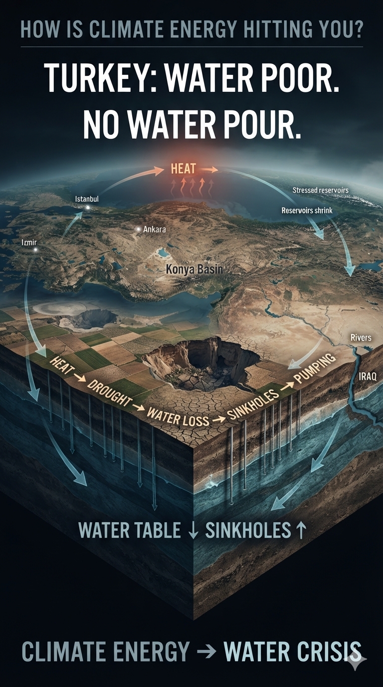
Türkiye is rapidly approaching a critical threshold at which it could officially become a water-poor nation by 2030, driven heavily by severe climate change and extensive groundwater mismanagement.
Located within the highly vulnerable Mediterranean Basin, Türkiye is experiencing plunging per-capita water availability, escalating drought, and an alarming 88 percent risk of nationwide desertification. The consequences extend far beyond water supplies. According to a climate assessment by the World Bank, a mere 10 percent reduction in water supply could cost the country 6 percent of its total GDP.
The emerging crisis illustrates how climate energy can propagate through an interconnected system: rising temperatures intensify drought; drought reduces surface water and reservoir replenishment; declining water supplies increase groundwater extraction; falling water tables destabilize the landscape; and the resulting agricultural, urban, and economic stresses compound one another.
Drivers of Water Poverty
Plunging Per-Capita Water Supply
The United Nations Convention to Combat Desertification warns that population growth combined with rising temperatures will push Türkiye into official water poverty within years.
As the population grows while available water supplies decline, the amount of water available per person continues to fall. Climate change compounds the problem by increasing evaporation, intensifying drought, and placing additional pressure on already limited freshwater resources.
Vanishing Natural Lakes
Environmental experts report that more than 75 percent of Türkiye’s lakes have completely dried up over the past 60 years.
The disappearance of natural lakes represents more than the loss of individual bodies of water. Lakes function as components of larger regional hydrological systems, storing water and supporting agriculture, ecosystems, and communities. Their disappearance is another visible indicator of a system under increasing water stress.
Diminishing Rainfall
Recurrent droughts occur every few years, causing critical declines in surface runoff and reservoir replenishment.
As precipitation becomes less reliable and temperatures rise, the same amount of rainfall can produce less usable water. Higher evaporation rates remove more moisture from soils, reservoirs, and landscapes, while shortened snowmelt cycles further alter the timing and volume of downstream water.
The Agriculture and Sinkhole Crisis
Groundwater Over-Extraction
As drought intensifies, farmers have increasingly turned to groundwater to sustain crops. An estimated 120,000 unlicensed wells have been dug to compensate for declining surface-water availability.
Groundwater therefore becomes a critical emergency reserve—but continued extraction faster than natural recharge transforms that reserve into a rapidly depleting resource.
Receding Water Tables
Heavy agricultural siphoning is causing underground water tables in central regions to decline by up to 16 feet annually.
This represents a profound alteration of the subsurface water system. As groundwater is removed faster than it can be replenished, the water table retreats deeper beneath the agricultural landscape.
Proliferating Sinkholes
The structural consequences are increasingly visible.
This underground depletion has contributed to the formation and collapse of more than 680 massive sinkholes across the crucial Konya Basin agricultural region.
The sinkholes provide a dramatic physical manifestation of the water crisis: what is being removed from beneath the landscape eventually manifests at the surface.
Urban and Geopolitical Strains
Stressed Mega-Cities
Major urban centers—including Istanbul, Ankara, and Izmir—face severe water scarcity as major reservoirs regularly fall below critical capacity.
The crisis is therefore not confined to rural agricultural regions. As water supplies tighten, cities must compete with agriculture, industry, ecosystems, and other demands for an increasingly constrained resource.
Downstream River Depletion
Shorter mountain snowmelt cycles are heavily reducing the natural volumes flowing into regional rivers.
Changes in snowpack and melt timing can disrupt the seasonal delivery of freshwater downstream, further stressing rivers, reservoirs, agriculture, and communities dependent upon predictable water flows.
Geopolitical Tensions
The water crisis also extends beyond Türkiye’s borders.
Restricted flows from dams on the Tigris and Euphrates rivers worsen severe water crises downstream in Syria and Iraq, according to The Water Project.
Water scarcity can therefore become a regional geopolitical problem, transforming climate-driven hydrological changes into competition among nations sharing increasingly stressed river systems.
The Climate-Energy Connection
Türkiye’s emerging water crisis demonstrates how climate energy does not remain confined to a thermometer reading.
Climate change increases the energy available to the atmosphere and intensifies the hydrological cycle. The resulting extremes can simultaneously increase evaporation, alter precipitation, accelerate snowmelt, reduce water availability, and increase demand for irrigation.
When human water consumption is added to those climate stresses, the system can move rapidly toward a critical threshold.
Water poor. No water pour.
For Türkiye, the question is no longer simply whether climate change will affect water availability. The emerging question is how quickly multiple water-related stresses can begin comingling and amplifying one another—and what happens when a nation’s agricultural, urban, economic, and geopolitical systems all depend upon the same shrinking resource.
Coastal Erosion, Property Loss & the Uninsurable Coast
Nicolas Cage: Whole Sinkhole
On September 8, 2026, severe coastal erosion and high surf triggered by the aftermath of Hurricane Marie caused the driveway of Nicolas Cage’s $10.5 million beachfront mansion to completely collapse.
The resulting crater expanded to roughly 30 by 60 feet and plunged about 25 feet deep, swallowing the driveway, a construction-site portable restroom, and heavy concrete debris.
Powerful south swells, extreme high tides, and pounding waves from Tropical Storm/Hurricane Marie ate away at the coastline directly beneath the property.
The collapse ruptured a gas main, forcing utility crews to shut off natural gas along the street. Because the ground remained highly unstable, city officials declared a local state of emergency and red-tagged or ordered evacuations for roughly 30 surrounding homes. Fortunately, the home was unoccupied at the time, and no injuries were reported.
California’s Coastal Erosion
Climate change and coastal erosion are fundamentally reshaping California’s 1,100-mile coastline. What was once considered a slow-moving, long-term environmental shift has accelerated into a series of highly disruptive events, resulting in collapsing bluffs, shrinking beaches, and massive infrastructure vulnerabilities.
The severe impacts California is facing are driven by a combination of rising sea levels and intensifying ocean patterns.
1. Vanishing Beaches and the “Coastal Squeeze”
California’s famous sandy beaches are facing an existential crisis. The U.S. Geological Survey (USGS) estimates that 24% to 75% of California’s beaches could completely erode by the year 2100.
The Squeeze: Normally, a beach would naturally migrate inland as sea levels rise. However, much of California’s coast is experiencing a “coastal squeeze”: beaches are trapped between the rising ocean and human-made infrastructure such as seawalls, highways, and residential developments, leaving the sand nowhere to go.
Artificial Interventions: According to recent USGS satellite data, some Southern California beaches have artificially expanded, but this is entirely due to expensive human interventions, such as dredging and “beach nourishment” projects, rather than natural coastal resilience.
2. Sea Cliff Failures and Deadly Landslides
Roughly 70% of California’s coast is comprised of oceanfront bluffs and cliffs.
Increased Wave Attack: As baseline sea levels rise, waves strike the base of these cliffs more frequently and with greater force. This severely degrades their structural stability, triggering sudden and unpredictable cliff collapses and landslides.
Human and Property Risk: Bluff failures have turned deadly for beachgoers in areas such as Encinitas and San Francisco. They also pose an immediate threat to multi-million-dollar cliffside homes and vital transportation routes.
3. The “Triple Threat” of El Niño and Severe Storms
While climate change is steadily raising the global baseline sea level, seasonal weather anomalies can trigger immediate emergencies. Geomorphologists at the Scripps Institution of Oceanography warn that El Niño conditions create a devastating “triple threat”:
Elevated Ocean Height: El Niño patterns can temporarily push local sea levels up by an additional 6 to 13 inches. Combined with pre-industrial sea-level rise, this radically amplifies the baseline ocean height.
Powerful Swells: Stronger storms and intense wave energy eat away at protective sand berms at an accelerated rate.
Heavy Rain: Atmospheric rivers saturate coastal land, triggering landslides from the top down while waves batter the cliffs from the bottom up.
The compound effect of these forces was highly visible during recent extreme-weather events, which caused widespread flooding in Long Beach and massive coastal sinkholes in Malibu. Every 2 to 4 inches of sea-level rise effectively doubles coastal flood risks.
4. Compounding Economic and Ecological Damages
Infrastructure at Risk: The state’s Legislative Analyst’s Office estimates that $8 billion to $10 billion worth of existing property could be entirely underwater within the next few decades, with billions more at risk during high tides. Critical lifelines—including the Pacific Coast Highway and coastal rail links such as the Amtrak lines connecting San Diego to Los Angeles—frequently face service suspensions because of ground instability.
Ecological Degradation: California has already lost more than 60% of its historical coastal sand dune systems to development and erosion. This destroys critical habitats for native birds and mammals while removing the coastline’s natural buffer against storm surges.
Water Supply Risks: Rising tides put freshwater aquifers at risk of saltwater intrusion. Increased saltwater contamination in the Sacramento-San Joaquin Delta threatens the drinking-water supply for millions of Californians as well as adjacent agricultural land.
California’s Adaptive Strategy
In response, California passed legislation such as Senate Bill 272, requiring all local governments within the coastal zone to establish comprehensive sea-level-rise plans by January 1, 2034. Communities are forced to choose between “hard armoring”—building massive rock revetments and groins to hold back the sea—and “managed retreat,” the highly controversial process of moving structures and infrastructure entirely inland.
Florida Coastal Erosion
Florida is facing a systemic coastal real-estate crisis in which climate-driven physical erosion has collided with aggressive new legal and financial mandates.
The state is experiencing severe physical land loss, but the downstream financial impact—specifically skyrocketing condo fees, massive special assessments, and a plunging condo market—is reshaping the state’s housing economy.
Part 1: How Coastal Erosion Is Impacting Florida
Florida features a low-lying, highly vulnerable topography. Rising sea levels and climate-fueled hurricanes are causing severe coastline degradation.
Critical Erosion: The Florida Department of Environmental Protection has designated a majority of Florida’s coastline as facing “critical erosion risk.” Beaches and barrier islands are shrinking, eliminating natural buffers that protect buildings from storm surges.
Foundation Undermining: Storm surges and intense wave action systematically wash away sand beneath seawalls and structural slabs. Saltwater intrusion aggressively corrodes the steel rebar inside concrete foundations and parking garages, severely compromising structural integrity over time.
Boundary Shrinkage: Coastal erosion is shrinking the physical legal boundaries of private properties. By 2050, over 140,000 Florida properties are expected to be significantly altered by land loss.
Part 2: The Condo Crisis — Fees & Special Assessments
Historically, beachfront condo associations kept their Homeowners Association (HOA) fees artificially low by voting to “waive” reserve funding for long-term maintenance. The tragic 2021 collapse of Champlain Towers South in Surfside permanently ended this practice.
Following the disaster, Florida passed strict safety laws, including SB 4-D and subsequent updates such as HB 913, creating a financial perfect storm:
Mandatory Milestone Inspections: All buildings three stories or taller that reached 30 years of age—or 25 years if within three miles of the coast—were required to complete rigorous structural inspections. These inspections uncovered decades of hidden saltwater corrosion, concrete spalling, and foundation rot.
Structural Integrity Reserve Studies (SIRS): Associations must perform a SIRS to calculate the remaining lifespan of critical components such as roofs, foundations, and load-bearing walls.
The Ban on Waiving Reserves: Associations are strictly prohibited from waiving or underfunding reserves for structural items. They must collect the required cash.
The Financial Fallout
Six-Figure Special Assessments: Because buildings deferred maintenance for decades, unit owners are being hit with mandatory, one-time special assessments ranging from $50,000 to more than $400,000 per unit to pay for multi-million-dollar structural repairs.
Skyrocketing Monthly Fees: Regular monthly HOA fees have surged—sometimes by 20% to 50% in a single year—to cover ongoing reserve requirements and exploding commercial-property insurance premiums.
Surging Insurance Costs: Driven by storm damage and climate risk, many major private insurers have pulled out of Florida entirely. Condo buildings are forced onto high-cost, bare-minimum state-backed policies, adding thousands of dollars annually to an individual unit owner’s bottom line.
Part 3: Devastation of Real Estate Values
The financial strain of these assessments and fees has broken the economics of Florida condo ownership, resulting in a dramatic price correction along the coast.
The Mass Sell-Off: Fixed-income retirees and middle-class owners cannot afford a sudden $100,000 assessment or a doubling of their monthly dues. This has caused a massive influx of inventory as desperate owners try to unload their units before deadlines hit.
Evaporating Buyer Demand: Disclosures showing thousands of non-compliant buildings, paired with high risk, have terrified buyers. Buyers refuse to inherit pending six-figure structural repair bills, causing sales velocity to freeze.
Deep Price Disruption: According to market trackers, this massive supply glut and lack of demand has led to steep price drops for coastal condos. In stark contrast to single-family homes, aging coastal condos are seeing values plummet by 20% to 40%.
Coastal Gentrification: The ultimate trajectory is severe economic displacement. As middle-class owners are forced out, developers and wealthy buyers are buying up entire distressed buildings at steep discounts, either to demolish them or completely rebuild luxury projects out of pocket.
Australia Coastal Erosion
Over 250,000 Australian homes are at risk of coastal erosion, according to the “Rising Seas, Rising Bills” report published by the Climate Council on September 10, 2026.
Drawing on groundbreaking climate modeling from the University of Melbourne and the Australian National University, the report highlights the severe threat that rising sea levels and storm surges pose to Australia’s massive coastal population.
1. The Real Estate and Financial Risk
Properties Threatened: The report explicitly warns that more than 267,000 coastal properties—roughly a quarter of a million homes—are at risk of severe inundation and erosion damage by 2100.
The $855 Billion Economic Bill: Total economic losses are projected to hit at least $855 billion AUD by the end of the century. This includes $274.3 billion AUD in direct property damage, alongside $580.7 billion AUD in damage to farmland, nature reserves, and critical public infrastructure.
The Timeline: While 2100 is the benchmark for the worst damages, researchers stress that the economic shock waves will start crippling coastal real estate as early as 2040.
2. State-by-State Breakdown: Where Is Most Exposed?
The damage is not distributed evenly, with specific regions carrying extreme structural and financial burdens:
Queensland — 93,157 properties at risk: The worst-affected state by property count. The Gold Coast alone is officially named Australia’s most exposed urban area, facing a staggering $84.4 billion AUD in projected economic losses on its own.
New South Wales — 71,210 properties at risk: Communities in Northern NSW and the Central Coast are projected to experience far higher property losses than Greater Sydney.
Western Australia — 51,366 properties at risk: While it has fewer homes at risk than Queensland or New South Wales, Western Australia faces the highest overall financial loss, at $230.5 billion AUD, due to vast tracts of highly valuable coastal agricultural land that will be permanently lost to sea-level rise.
Victoria: Property losses are heavily concentrated in low-lying, densely populated urban areas around Melbourne’s Port Phillip Bay and the Yarra River.
3. The Uninsurable “Actions of the Sea”
Much like the condo crisis unfolding in Florida, Australia is facing a severe insurance reckoning.
The Exclusion Clause: Most standard private insurers in Australia explicitly exclude coverage for “actions of the sea.” This means regular ocean tidal flooding, steady coastal erosion, and sea-level rise are completely uncovered.
The Cost Burden: When a storm surge destroys a foundation or a cliff collapses, property owners will largely be forced to bear the multi-million-dollar stabilization or relocation costs entirely on their own. Experts warn that this will trigger massive drops in property values and result in “uninsurable” coastal ghost zones.
The Coast Is Becoming a Financial Fault Line
From California to Florida to Australia, coastal erosion is no longer simply a problem of disappearing sand or retreating shorelines. It is becoming a cascading climate-energy problem that reaches directly into property values, insurance markets, infrastructure, ecosystems, and household finances.
The Nicolas Cage sinkhole provides a dramatic example of how quickly coastal instability can turn an expensive piece of real estate into a dangerous hole in the ground. California demonstrates the growing physical vulnerability of beaches, cliffs, transportation corridors, and freshwater resources. Florida shows how physical climate risks can cascade into insurance crises, special assessments, and collapsing real-estate economics. Australia demonstrates how the same process can scale into a national financial exposure measured in hundreds of billions of dollars.
The underlying lesson is straightforward: coastal climate risk does not stop at the water’s edge.
As sea levels rise and extreme coastal events intensify, the physical loss of land can propagate through the economic system. Erosion undermines structures. Structural damage increases repair costs. Repair costs increase insurance premiums and assessments. Insurance becomes unavailable or unaffordable. Properties lose value. Buyers disappear. Communities face declining tax bases and increasingly expensive infrastructure protection.
What begins as coastal erosion can therefore become a cascading economic feedback.
Climate energy is hitting the coast—and increasingly, it is hitting the balance sheet.