Sea-Level Rise: Rubbing Salt in the Wound

Posted on 2026/08/232026/08/23 by admin

by Daniel Brouse and Sidd Mukherjee

How Is Climate Energy Hitting You?

The Jersey Shore Is Sure

Sea-Level Rise: Rubbing Salt in the Wound

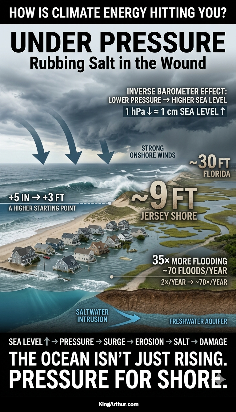
Sea-level rise is not simply a matter of the ocean getting higher. Climate change is altering the physical forces that move water toward and onto the shoreline. Rising seas, changing atmospheric pressure, stronger winds, altered ocean circulation, storm surge, king tides, and saltwater intrusion can interact to turn gradual sea-level rise into a much more immediate coastal threat.

A Real-World Warning: The Wetlands Institute

The experience of The Wetlands Institute in Stone Harbor, New Jersey, provides a striking example of how quickly coastal conditions can change.

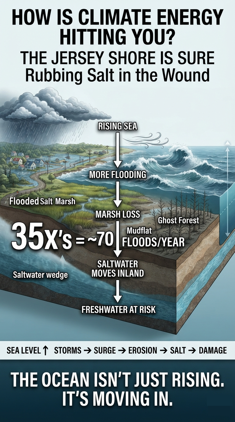
The institute’s Salt Marsh Trail reportedly flooded only a few times a year around 2000. Over the past five years, flooding has averaged nearly 70 times annually. The institute is closing its headquarters on September 7, 2026, to begin a major coastal-resilience transformation.

The response includes raising the Salt Marsh Trail by two to three feet using clean dredged material, temporarily relocating operations and educational programs, and pursuing a broader campaign to replace and elevate the existing campus buildings.

This is more than an inconvenience. Increasingly frequent inundation can fundamentally alter the coastal ecosystem itself.

The Climate Shift

Accelerated sea-level rise: Sea levels along parts of the New Jersey coast are rising faster than the global average.
Marsh degradation: Repeated inundation can overwhelm salt-marsh vegetation, converting productive marsh into mudflats and eventually open water.
Wildlife disruption: More frequent flooding threatens habitats used by marsh-dependent birds and can interfere with diamondback terrapin nesting.
Infrastructure exposure: Roads, buildings, trails, drainage systems, and utilities face increasingly frequent flooding even without a major storm.

The critical point is that the climate signal is not experienced as a smooth, uniform rise in water level. It is experienced as more frequent encounters with water.

1. The Inverse Barometer Effect: Atmospheric Pressure Pushes the Ocean

Atmospheric pressure exerts physical force on the ocean surface. When a deep low-pressure system moves over the coast, the reduced atmospheric weight allows the ocean surface to rise.

The approximate relationship is:

A 1-hectopascal (hPa) decrease in atmospheric pressure produces roughly a 1-centimeter rise in sea level.

A very deep storm can therefore raise the local ocean surface substantially before the effects of wind-driven storm surge are even considered.

This is known as the inverse barometer effect.

Climate change does not simply “raise the sea.” It can alter the atmospheric conditions that determine how that elevated ocean is distributed along the coastline at any particular moment.

Inverse Barometer Effect Examples

Storm type	Approx. pressure near coast	Pressure drop from 1013 hPa	Inverse-barometer rise
Ordinary coastal storm	990–1000 hPa	13–23 hPa	5–9 in
Strong nor’easter	970–985 hPa	28–43 hPa	11–17 in
Very strong coastal storm	950–965 hPa	48–63 hPa	19–25 in
Sandy-type extreme	~945 hPa	~68 hPa	~27 in / 2.2 ft
Exceptional low-pressure event	930–940 hPa	73–83 hPa	29–33 in / 2.4–2.8 ft

The Combined Impact

The inverse barometer effect combines with wind stress, coastline shape, bathymetry, wave setup, tides, and storm track can produce much larger water-level changes. Hurricane Sandy’s actual coastal water levels were dramatically higher because the pressure effect was combined with enormous wind-driven surge, wave action, tide, and the storm’s exceptionally favorable track. At Sandy Hook, water reached about 8.9 feet above ground level, while the storm produced major surge throughout the central and northern Jersey Shore.

An additional 5 inches to 3 feet of sea-level rise represents a new baseline of climate energy impacting coastal communities. The inverse barometer effect then combines with wind stress, coastline shape, bathymetry, wave setup, tides, and storm track to produce much larger water-level changes. The result can be extreme coastal flooding, with observed water levels reaching roughly 9 feet above ground level along parts of the Jersey Shore and as much as 30 feet in parts of Florida during major storms.

2. Wind and Wave Energy: Turning Pressure Gradients Into Coastal Damage

Atmospheric pressure gradients—the differences between areas of high and low pressure—drive winds.

When those gradients become stronger, winds can become stronger and more persistent. Strong winds transfer energy to the ocean, generating larger waves and increasing wind setup, the piling of water against the coast.

The consequences can include:

Higher water levels along exposed shorelines
Larger and more destructive waves
Increased dune erosion
Offshore transport of beach sand
Overtopping of coastal defenses
Greater storm-surge penetration

The shoreline therefore experiences not only a higher baseline sea level but also increasingly energetic ways of moving that water around.

3. Altered Ocean Circulation: When Water Piles Up

Changes in large-scale atmospheric circulation can alter ocean currents and regional sea levels.

The relationship between the Gulf Stream, the North Atlantic circulation, winds, and coastal sea level is particularly important along the U.S. East Coast. Changes in ocean circulation can redistribute enormous volumes of water, producing dynamic sea-level changes that may differ substantially from the global average.

In simplified terms, when ocean circulation changes, water can accumulate against a coastline rather than being transported away from it.

That means a community can experience a rapid increase in local relative sea level even when the global mean is changing much more slowly.

4. Compound Coastal Flooding: When Everything Arrives Together

The most dangerous coastal flooding occurs when multiple processes reinforce one another.

Imagine a high tide occurring while:

Global sea level is already elevated.
A low-pressure storm raises the ocean through the inverse barometer effect.
Strong onshore winds push additional water toward land.
Large waves increase water levels and erode dunes.
Heavy rainfall overwhelms drainage systems.
Rivers are already elevated and cannot discharge efficiently.

These processes can combine into compound flooding.

The problem is not simply that the water is higher. The problem is that multiple pathways for moving water onto the land are operating simultaneously.

Salt marshes normally provide a natural buffer. But repeated inundation and erosion can eventually overwhelm the marsh itself. Once protective wetlands deteriorate, more wave energy reaches infrastructure, creating a feedback loop of increasing exposure and increasing damage.

Saltwater Intrusion: When the Ocean Moves Underground

Sea-level rise has another consequence that is much less visible than coastal flooding: saltwater intrusion.

Saltwater intrusion occurs when seawater moves into freshwater systems, including groundwater aquifers, rivers, wetlands, agricultural soils, and drinking-water supplies.

Two forces are especially important:

Rising sea level increases the hydraulic pressure and inland reach of seawater.
Drought and reduced groundwater recharge weaken the freshwater pressure pushing outward toward the sea.

Together, these forces can shift the boundary between freshwater and saltwater inland.

Research has projected that saltwater contamination could affect a very large proportion of coastal aquifers by 2100, although the extent varies substantially by geography, aquifer characteristics, groundwater use, and future climate conditions.

How the Saltwater Wedge Moves Inland

Under normal conditions, rainfall replenishes groundwater. Freshwater flows toward the coast and maintains a hydraulic gradient that helps resist seawater intrusion.

Because freshwater is less dense than seawater, a freshwater lens can exist above denser saltwater beneath coastal areas.

But the balance can shift.

1. Underground Aquifer Intrusion

As sea level rises, the hydraulic pressure exerted by seawater increases. At the same time, climate-driven drought and higher temperatures can reduce groundwater recharge in some regions.

Less freshwater flowing toward the ocean means less outward pressure resisting seawater.

The underground saltwater boundary can therefore migrate inland.

This process can occur largely out of sight until a well begins producing water with elevated salinity.

2. Surface and Vertical Infiltration

Storm surge, king tides, and coastal flooding can push seawater onto land.

If that water remains on the surface, it can infiltrate downward through soils and shallow geological formations, contaminating groundwater.

Repeated flooding is especially important because a single event may be temporary, while dozens of inundation events each year can progressively alter soil and groundwater chemistry.

3. The “Highway Effect”

Human modifications to coastal landscapes can provide pathways for seawater to travel inland.

Agricultural drainage ditches, shipping channels, tidal creeks, canals, and other engineered waterways can connect coastal waters with areas that were historically protected by natural terrain.

When sea level rises or storm surge moves inland, these channels can function as highways for saltwater.

The Ecological and Economic Consequences

Saltwater intrusion does not stop at the shoreline.

Ghost Forests

As saltwater enters coastal soils and groundwater, freshwater-dependent trees can die from prolonged salt stress. The result can be stands of dead trees known as ghost forests.

These landscapes provide visible evidence that the boundary between marine and terrestrial ecosystems is moving inland.

Agricultural Damage

Salt deposited on agricultural land can accumulate in the root zone.

Excessive soil salinity interferes with plants’ ability to absorb water and can reduce crop productivity. Persistent salinization can make valuable coastal farmland increasingly difficult—or eventually impossible—to farm without expensive remediation and freshwater management.

Infrastructure Corrosion

Saltwater and brackish groundwater are highly corrosive.

Repeated exposure can accelerate deterioration of underground pipes, electrical infrastructure, concrete, foundations, roads, and other infrastructure.

The damage can occur beneath the surface long before it becomes visually obvious.

Drinking-Water Threats

Coastal communities that depend on groundwater face a particularly serious vulnerability.

Pumping already lowers groundwater levels around wells. If the freshwater table is lowered too far, the hydraulic gradient resisting seawater intrusion weakens further.

This can create another feedback:

More pumping → lower freshwater pressure → greater saltwater intrusion → less usable freshwater.

The Larger Picture: Climate Energy Does Not Disappear

Sea-level rise is one expression of a much larger physical process.

The additional energy accumulating in the climate system does not simply produce a higher average temperature. Energy moves through the atmosphere, ocean, land, ice, and biosphere.

Along the coast, that energy can appear as:

Higher baseline sea level → more frequent tidal flooding → stronger storm impacts → erosion → wetland loss → saltwater intrusion → infrastructure damage → freshwater stress.

The critical distinction is between average conditions and actual events.

A few inches of average sea-level rise may sound modest. But those inches can determine whether a high tide remains below a road or flows across it. They can determine whether a storm surge is absorbed by a functioning marsh or reaches buildings and infrastructure.

The climate system does not deliver its additional energy evenly.

It delivers it through water, wind, waves, heat, storms, erosion, flooding, and ecological disruption.

And along the coast, the ocean is increasingly finding more ways to come ashore—and stay there.

Where’s the Beef? Tariffs, Inflation, and the Climate Cost of Meat

Posted on 2026/08/21 by admin

On August 21, 2026, President Donald Trump announced a temporary 90-day waiver of out-of-quota tariffs on imported ground beef, allowing up to 300,000 metric tons to enter the U.S. market tariff-free in an effort to reduce grocery prices. The president said he had secured a commitment that the imported meat would be sold at 25% below current market prices, providing relief from persistent food inflation.

The move is intended to address a dramatic increase in the cost of ground beef, which has risen roughly 57% over the past five years. But the policy immediately drew backlash from domestic cattle ranchers and rural-state Republicans, including Senator Tim Sheehy, who warned that flooding the market with cheaper foreign beef could undermine American cattle producers.

There is another problem that may be even more important to consumers: much of the imported beef affected by the policy is frozen beef destined for commercial and restaurant use, rather than the fresh ground beef consumers typically purchase at the grocery store. That means the immediate impact on household grocery bills may be considerably smaller than the headline numbers suggest.

More importantly, the tariff waiver does little to address the underlying forces driving higher beef prices.

Climate Change Is Becoming an Inflation Problem

The cattle industry is increasingly exposed to the economic consequences of climate extremes. Drought, extreme heat, wildfires, water scarcity, degraded pasture, and volatile feed supplies all increase the cost of raising cattle. When these pressures become severe enough, ranchers may be forced to reduce their herds, further constraining beef supplies and pushing prices higher.

This creates a feedback loop. Climate extremes increase production costs and reduce the supply of cattle. Reduced supply raises beef prices. Higher prices then encourage producers to rebuild their herds, but rebuilding takes years. Another drought or extreme-weather event during that process can once again force herd reductions.

This is why simply importing cheaper beef may treat the symptom without addressing the disease.

The larger economic issue is what I call climate inflation: the gradual—and increasingly rapid—incorporation of climate-related costs into the prices of food, energy, insurance, housing, transportation, and other necessities.

For the past several years, inflation discussions have focused primarily on monetary policy, supply chains, labor costs, tariffs, and government spending. Those factors certainly matter. But climate-driven disruptions are becoming an increasingly important component of the cost structure of the economy.

And unlike a temporary tariff or a change in interest rates, climate pressures can compound over time.

The Beef Problem Is Bigger Than Beef

A 90-day tariff waiver may provide some temporary relief. It may even benefit restaurants and commercial food purchasers if imported frozen beef reaches the market at substantially lower prices.

But it does not create more water, restore drought-stricken grazing land, prevent wildfires, reduce extreme heat, or rebuild cattle herds that have been lost to climate-driven conditions.

Nor does it address the increasingly expensive insurance, infrastructure, agricultural, and supply-chain consequences of a changing climate.

If climate extremes continue to intensify, we should expect more of these conflicts. Policymakers will repeatedly face the same choice: temporarily suppress prices by opening markets to cheaper imports, or address the underlying conditions that are making domestic production increasingly expensive.

Where’s the beef?

It may increasingly be somewhere else.

And that is the larger warning. Climate change is no longer simply an environmental issue. It is becoming an economic variable—and climate inflation may prove to be one of the most consequential economic developments of the next decade.

Treasury Doubles Bond Buybacks as U.S. Bond Market Volatility Deepens

Posted on 2026/08/202026/08/21 by admin

The U.S. Department of the Treasury intervened on August 19, 2026, announcing that it will at least double the size of its liquidity-support bond buyback operations in an effort to calm a highly volatile Treasury market.

Under the direction of Treasury Secretary Scott Bessent, the maximum repurchase limits for longer-dated nominal coupon securities will increase from $2 billion to at least $4 billion per operation. The larger limits, covering the 10- to 20-year and 20- to 30-year sectors, are scheduled to take effect September 9 and remain in place through November 4, 2026.

The intervention followed a prolonged “buyers’ strike” in the Treasury market that pushed the 30-year Treasury yield to approximately 5.34%—its highest level since 2007. Concerns surrounding persistent inflation, the prospect of war with Iran, heavy borrowing by the artificial-intelligence sector, and the U.S. national debt surpassing the $40 trillion threshold have contributed to growing pressure on longer-term government bonds.

The Treasury announcement produced an immediate market response. Bond prices rallied, while the 30-year Treasury yield fell by nearly 10 basis points to approximately 5.19%. Major Wall Street stock indexes also rebounded as investors responded to the prospect of increased liquidity and stability in the Treasury market.

A Troubling Signal

While Treasury describes the expanded buybacks as a liquidity-support measure, the intervention raises a broader question: How much government intervention should occur in what is supposed to be a private, market-driven financial system?

The Treasury market is the foundation of the U.S. financial system. When the government becomes an increasingly active participant in supporting the market for its own debt, it can create the perception that market forces are no longer being allowed to fully determine the price of that debt.

That is concerning not only for investors, but also for citizen-taxpayers. Ultimately, the federal government is supporting a debt market built upon obligations that taxpayers are responsible for financing.

The market’s reaction is therefore significant. The immediate rally may provide short-term relief, but the underlying pressures— inflation, enormous federal borrowing, rising interest costs, geopolitical risk, and declining demand for long-term Treasury securities—remain.

Government intervention may calm the market temporarily. It does not eliminate the underlying risks.

When the government has to step into its own debt market to provide liquidity, the intervention itself becomes a market signal—and the bond market has reacted accordingly.

UPDATE

After I wrote the bond article, Scott Bessent appeared live on CNBC for an interview. He doubled down on the Treasury’s intervention in the bond market, apparently because the market did not react strongly enough to his initial announcement. He emphasized that $4 billion per operation is now the minimum baseline for Treasury buybacks.

The good news? The Treasury doesn’t have that much money available to keep buying back bonds.

The Bleeding Edge of Climate Change

Posted on 2026/08/192026/08/19 by admin

by Daniel and Sidd

While Sidd was in town, I took some notes. Somehow, they turned into this:

Climate Change: The Big Picture

There are many ways to look at climate change. From a micro perspective, there are millions of individual feedbacks operating throughout the Earth system. From a macro perspective, there is the climate system as a whole.

Understanding how those feedbacks interact—and, more importantly, how they feed back into one another—is at the bleeding edge of climate science.

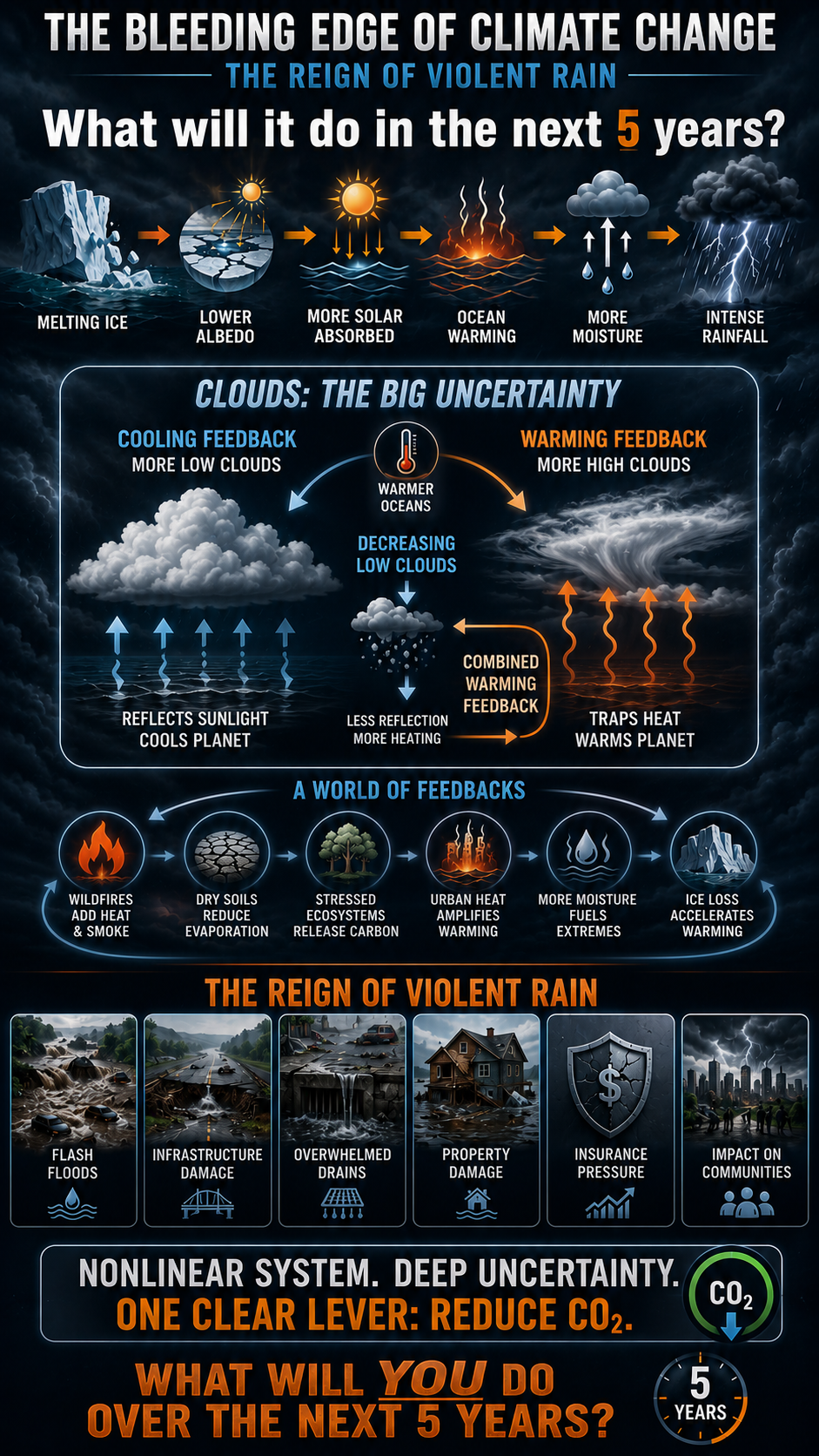
One of the simplest examples is the albedo effect. The physics of ice is straightforward: bright, reflective ice sends a portion of incoming solar energy back into space, while darker ocean absorbs it. Less ice means more absorbed energy and, therefore, more warming.

But the system quickly becomes much more complicated.

How does changing albedo affect cloud formation, particularly over the tropics? And what happens to the climate if those clouds increase—or decrease?

The low clouds are especially important. They can reflect substantial amounts of incoming sunlight back into space. If tropical low clouds diminish, the ocean could absorb significantly more solar energy, accelerating warming.

This is where the bleeding edge begins.

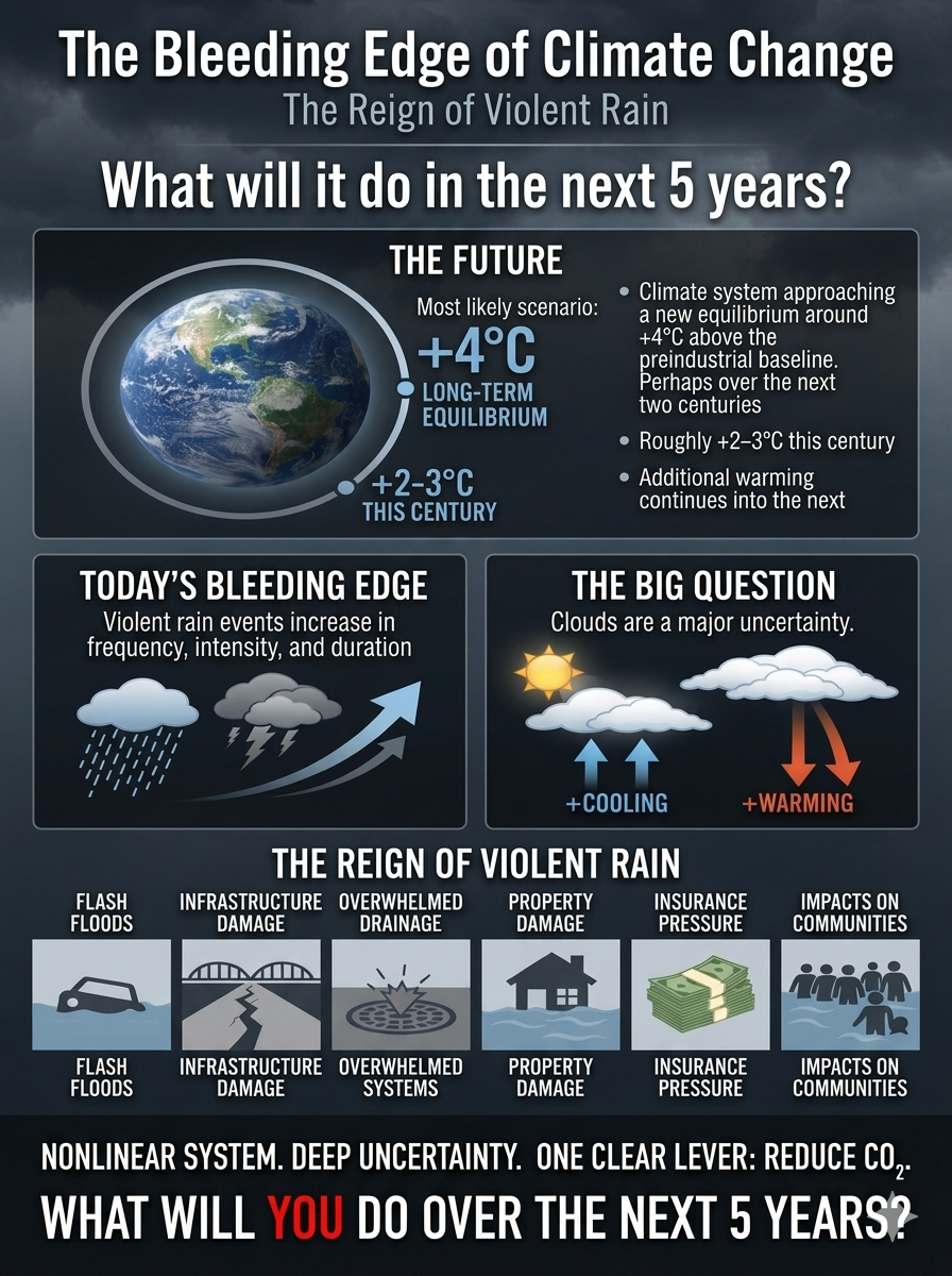
Clouds are arguably the largest remaining uncertainty in our understanding of climate sensitivity. They can both reflect incoming solar radiation and trap outgoing heat. Which effect dominates—and how that balance changes as the planet warms—is one of the great questions in climate science.

My expectation is that the climate system could eventually approach a new equilibrium around +4°C above the preindustrial baseline, perhaps over the course of a couple centuries. That would imply roughly +2–3°C this century, with additional warming continuing into the next.

But that remains uncertain.

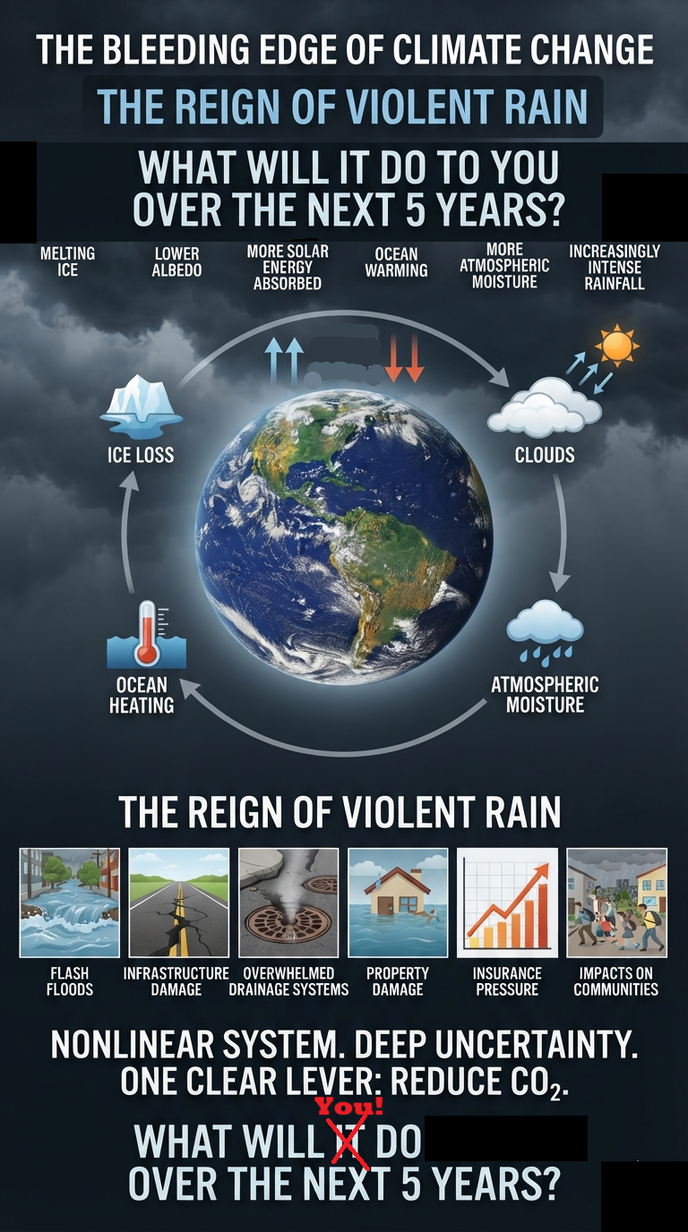
The important point is that climate change is not a simple linear equation. It is a massively interconnected system in which changes in one component can alter another, which then feeds back into the first. Ice affects albedo. Albedo affects heating. Heating affects clouds. Clouds affect radiation. Radiation affects ocean temperatures. Ocean temperatures affect evaporation and atmospheric moisture. And the cycle continues.

Everything is nonlinear.

Yet uncertainty about the exact trajectory does not mean uncertainty about what we should do.

The clearest lever we have is still the same: reduce CO₂ emissions and slow the accumulation of greenhouse gases in the atmosphere.

And while the long-term equilibrium matters, there is a much more immediate question.

What happens to you over the next five years?

We are already seeing rainfall becoming more intense and, in many places, more destructive—violent. A warmer atmosphere can hold more water vapor, increasing the potential for extreme precipitation. The question isn’t simply how hot the planet might become over the next 50 years.

The more immediate question is:

What is the violent rain going to do to your home, your community, your infrastructure, your insurance—and you—over the next five years?

That is where climate change stops being a distant projection and starts becoming a personal reality.

Demand Destruction: Bad News for the Economy, Good News for the Environment

Posted on 2026/08/14 by admin

U.S. retail sales fell unexpectedly by 0.6% month over month in July 2026, coming in well below the forecast of a 0.1% increase. The data, released this morning, points to a significant slowdown in American consumer spending and a reversal of the momentum seen in previous months.

Key Figures From the July Report

Headline retail sales: Down 0.6%, following a revised 0.2% increase in June.
Excluding autos: Down 0.3%, versus expectations for a 0.2% increase.
Excluding autos and gasoline: Down 0.2%, compared with an expected 0.3% increase.
Control group sales: Down 0.4%, missing the projected 0.3% gain.

Bad News for the Economy

The broad-based weakness suggests that American consumers are becoming increasingly constrained by high prices, elevated living costs, and strained household budgets. Discretionary spending appears to be particularly vulnerable as consumers cut back in response to declining purchasing power.

The slowdown is also affecting financial-market expectations, potentially strengthening the case for a more accommodative Federal Reserve monetary policy in the months ahead.

But there is another way to look at these numbers.

Demand Destruction

This may be another indication of demand destruction—a sustained reduction in consumption caused by rising prices, declining purchasing power, supply constraints, or the availability of alternatives.

Climate change can contribute to this process in several ways. Extreme heat, drought, flooding, wildfires, and other climate-related disruptions can damage agricultural production and supply chains, increasing the cost of food and other necessities. Rising insurance, energy, transportation, and infrastructure costs can further squeeze household budgets.

Food prices are particularly important. Climate-driven disruptions to agriculture can contribute to food inflation, creating one of the most direct ways climate change reaches the household budget. When essential goods become more expensive, consumers have less money available for discretionary purchases.

That creates an uncomfortable paradox.

Bad News for Consumers. Good News for the Climate?

For lower-income households, this is unquestionably bad news. Families already living close to the edge have far less ability to absorb higher food, housing, energy, transportation, and insurance costs. For them, demand destruction isn’t a lifestyle choice. It can mean doing without necessities or postponing purchases they would otherwise make.

But from an environmental perspective, declining consumption can have an unexpected benefit.

Our economy is built around a powerful cycle: produce more → sell more → consume more → produce even more. Economic growth has traditionally depended heavily on increasing consumption of energy, materials, goods, and services.

If rising costs begin breaking that cycle, the result could be a gradual decline in resource consumption.

That is the paradox of demand destruction:

What is bad news for the economy can sometimes be good news for the environment.

A reduction in fossil-fuel consumption, material throughput, unnecessary production, and resource-intensive consumption can reduce environmental pressures. In that sense, demand destruction could unintentionally contribute to the transition away from an economic model based on ever-increasing consumption.

The problem is that we should not confuse economic hardship with a successful environmental transition.

There is a profound difference between people consuming less because they have chosen more efficient, sustainable alternatives and people consuming less because they can no longer afford what they need.

The first represents managed transition.

The second represents contraction.

The challenge is to find a way to reduce humanity’s environmental footprint without forcing the people least able to absorb the costs to bear the greatest burden.

That may ultimately be one of the defining economic challenges of climate change: how do we move beyond consumerism without making poverty the mechanism that gets us there?

U.S. Fiscal Deficit Surges as 30-Year Treasury Yields Hit 25-Year High

Posted on 2026/08/13 by admin

by Daniel Brouse

The U.S. federal budget deficit reached a record $432 billion in July 2026, the largest deficit ever recorded for the month of July and the widest monthly shortfall since March 2021.

The July surge pushed the cumulative deficit for the first 10 months of fiscal year 2026 to approximately $1.8 trillion—already exceeding the $1.775 trillion deficit recorded for the entire 2025 fiscal year, with two months still remaining. The nonpartisan Congressional Budget Office (CBO) now projects the full-year FY2026 deficit could reach approximately $2.1 trillion.

At the same time, the cost of financing that debt is rising sharply.

Today’s $25 billion, 30-year Treasury bond auction is on track to clear at a yield of approximately 5.23%–5.24%, which would represent the highest yield on newly issued 30-year U.S. government debt since 2001.

The combination is significant: federal borrowing is accelerating while the market is demanding substantially higher compensation for holding long-term U.S. debt.

The elevated 30-year yield reflects a growing term premium—the additional return investors demand to compensate for the risks associated with holding long-duration government debt. Those risks include persistent fiscal deficits, rapidly expanding federal debt, inflation uncertainty, and the possibility that the supply of Treasury securities will continue to overwhelm demand at historically low yields.

This creates a potentially important feedback loop.

Larger deficits → more Treasury issuance → higher required yields → higher interest expense → larger future deficits.

The United States is therefore confronting two pressures simultaneously: the government is borrowing more, and borrowing is becoming more expensive.

A single month’s deficit does not establish a fiscal crisis. But the combination of a $432 billion July shortfall, an already $1.8 trillion fiscal-year deficit, a projected $2.1 trillion full-year gap, and long-term Treasury yields above 5% is an increasingly difficult fiscal equation.

The critical issue is no longer simply how large the federal deficit is.

It is how much more expensive it will become to finance it.

Money Moves People: Why Demand Destruction May Be the Fastest Path Beyond Fossil Fuels

Posted on 2026/08/132026/08/13 by admin

by Daniel Brouse

2026: The New Economic Reality

Money moves people.

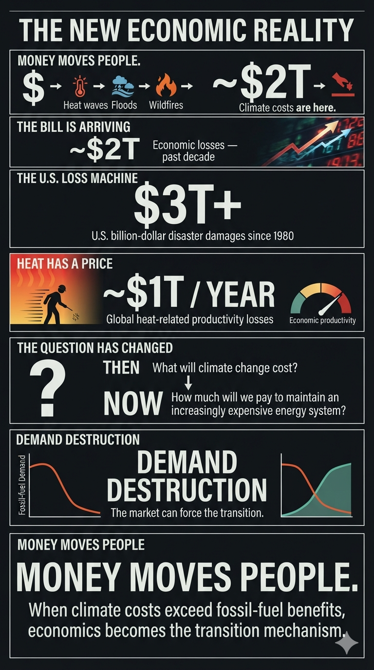
The climate costs of fossil-fuel dependence are increasingly outweighing its benefits—not in some distant future, but here and now. We are moving beyond arguments about what climate change might cost decades from today. Across the Western world, climate impacts are already imposing costs of hundreds of billions of dollars in real time.

Insurance is only one part of the story.

Infrastructure, agriculture, transportation, labor productivity, public health, energy systems, and financial markets are all beginning to absorb the cost of a destabilizing climate. The economic question is therefore changing. It is no longer simply:

“What will climate change cost us?”

It is increasingly:

“How much are we willing to pay to preserve an energy system that is becoming progressively more expensive to maintain?”

Climate Stress Is Becoming an Economic Stress Test

The physical infrastructure of the global economy is already being affected.

Maersk CEO Vincent Clerc has warned that climate change is putting increasing pressure on European waterways and that substantial infrastructure investment will be needed to keep the Rhine operating as a critical transportation artery.

But the economic importance of waterways extends far beyond shipping.

Rivers, lakes, and reservoirs are also critical components of the energy, industrial, agricultural, municipal, and ecological systems that support modern economies.

When water levels fall or water temperatures rise, power plants can be affected directly. Thermoelectric and nuclear power plants rely heavily on water for cooling. If river flows become too low, or water temperatures become too high, operators may be forced to reduce generation or temporarily shut down units because sufficient cooling capacity is no longer available or because thermal discharge limits are exceeded.

That creates an economic chain reaction:

Lower river flows or higher water temperatures
↓
Reduced cooling capacity
↓
Reduced power generation
↓
Tighter electricity supplies
↓
Higher electricity prices and grid stress
↓
Higher operating costs for industry and consumers

The same waterways that transport fuel, raw materials, agricultural products, chemicals, and manufactured goods can therefore also be essential to producing the electricity needed to move and manufacture those goods.

Water is simultaneously a transportation system, cooling system, industrial input, agricultural resource, and ecological asset.

When that system becomes unstable, multiple economic sectors can be affected at the same time.

Low water levels can also restrict the movement of coal, oil, natural gas, grain, chemicals, construction materials, and other bulk commodities. Barges may have to reduce their loads or make more trips to transport the same volume of goods. In some cases, alternative transportation by rail or truck becomes necessary, increasing fuel consumption, congestion, labor costs, and emissions.

Flooding creates the opposite problem.

Excess water can damage ports, locks, bridges, rail connections, roads, warehouses, industrial facilities, and electrical infrastructure. A waterway can therefore become economically disruptive at both extremes—too little water and too much water.

Agriculture is similarly exposed. Rivers and reservoirs provide irrigation, livestock water, and municipal supplies. Persistent drought can reduce agricultural output while increasing competition among farmers, cities, industry, ecosystems, and energy producers for increasingly scarce water.

There is also a less visible economic cost: water temperature itself is becoming an economic variable.

Warmer rivers can reduce their ability to absorb additional heat from industrial processes and power-plant cooling systems. At the same time, warmer water can stress aquatic ecosystems, fisheries, and drinking-water systems, creating additional regulatory, treatment, and ecological costs.

This produces a broader economic concept that is often missed in conventional disaster accounting:

Waterway disruption is not a single-sector problem. It is a systems problem.

The Rhine and Danube are not simply waterways. They are components of Europe’s economic infrastructure. They connect ports, factories, power plants, farms, cities, mines, warehouses, rail networks, and consumers. When climate conditions interfere with their operation, the economic consequences propagate through the system. A river does not have to disappear to create an economic crisis. It only has to become less reliable. And reliability is one of the most valuable—and often least visible—assets in a modern economy.

The Economic Toll of Extreme Weather

Global extreme weather and natural disasters are generating enormous economic losses. Recent estimates from the International Chamber of Commerce, insurers including Swiss Re, and disaster-loss tracking organizations show that severe convective storms, wildfires, floods, and other extreme events are producing annual losses measured in the hundreds of billions of dollars.

The first half of 2026 alone has already produced approximately $100 billion in global economic losses, while the cumulative economic toll over the past decade has reached roughly $2 trillion, according to recent assessments.

And the year is not over.

The second half of the year normally includes the peak of the North Atlantic hurricane season, creating the potential for another substantial wave of losses.

The Major Economic Drivers

Escalating annual losses.
Global disaster losses continue to accumulate at extraordinary levels. The combined economic losses from 2022 and 2023 alone have been estimated at roughly $451 billion.

The concentration of U.S. losses.
The United States remains a major source of global insured catastrophe losses. By June 2026, the country had already experienced 12 billion-dollar weather and climate disasters, with estimated losses totaling approximately $31.9 billion.

Severe convective storms.
Hail, tornadoes, straight-line winds, and other severe thunderstorms have become an increasingly persistent source of financial losses. The United States recorded a record 21 billion-dollar severe-convective-storm events in 2025.

Extreme heat and productivity.
The economic damage from climate change is not limited to destroyed buildings and infrastructure. Heat reduces worker productivity, particularly in construction, agriculture, manufacturing, and outdoor occupations. Global heat-related productivity losses have been estimated at roughly 1% of world GDP annually—around $1 trillion.

The long-term U.S. bill.
U.S. billion-dollar weather and climate disasters have generated cumulative damages exceeding $3 trillion since systematic tracking began in 1980.

The Trajectory Is the Story

Recent U.S. disaster statistics illustrate the increasing economic burden:

Year	Billion-Dollar Events	Estimated Damage	Major Loss Drivers
2025	23	~$115 billion	Severe storms, wildfires
2024	27	~$182.7 billion	Severe storms, tropical cyclones, extreme heat
2023	28	$145+ billion	Severe storms and other extreme events

The important point is not that every individual disaster can be attributed exclusively to climate change.

The economic signal emerges from the frequency, intensity, persistence, and cumulative cost of extreme conditions.

Climate change does not need to create every storm, flood, drought, or wildfire to transform the economics of risk. It only needs to increase the probability, severity, or duration of damaging events enough to alter the cost structure of society.

That is already happening.

“Demand Destruction” Is Our Friend

This brings us to one of the most powerful—and least appreciated—economic mechanisms in the energy transition:

Demand destruction.

The International Energy Agency has projected that global oil demand will decline more sharply than previously expected in 2026, forecasting a reduction of approximately 1.6 million barrels per day.

The significance extends beyond the number itself.

As an economist, I am less concerned with establishing a specific date by which the world must eliminate fossil fuels than I am with changing the economic forces that sustain fossil-fuel demand.

That distinction matters.

People do not necessarily change because someone wins an argument about climate science. They change because incentives change. Prices change. Risk changes. Availability changes. And eventually, behavior changes.

Money Moves People

I am unlikely to change the minds of the roughly 20% of Americans who are ideologically committed to policies that accelerate fossil-fuel dependence.

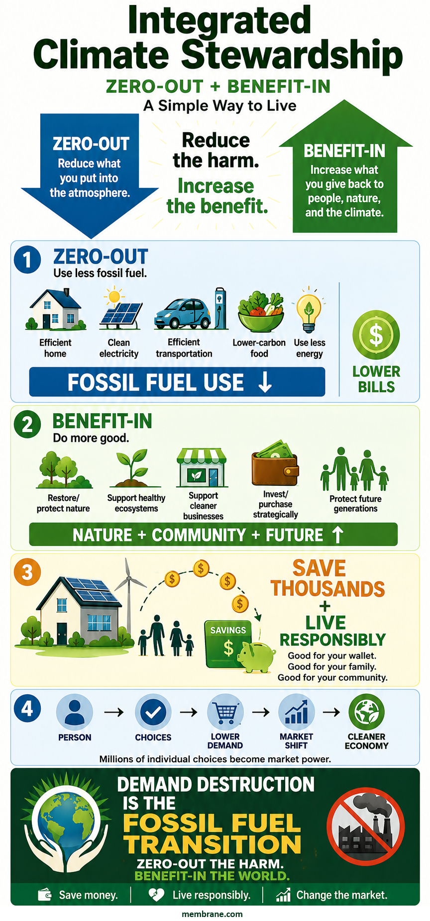
But that leaves the vast majority of the population. And economics can do much of the work. Integrated Climate Stewardship begins with reducing unnecessary consumption.

Consumerism drives energy demand, resource extraction, pollution, waste, and habitat destruction. Every unnecessary unit of consumption represents another demand for energy and materials somewhere in the global economy.

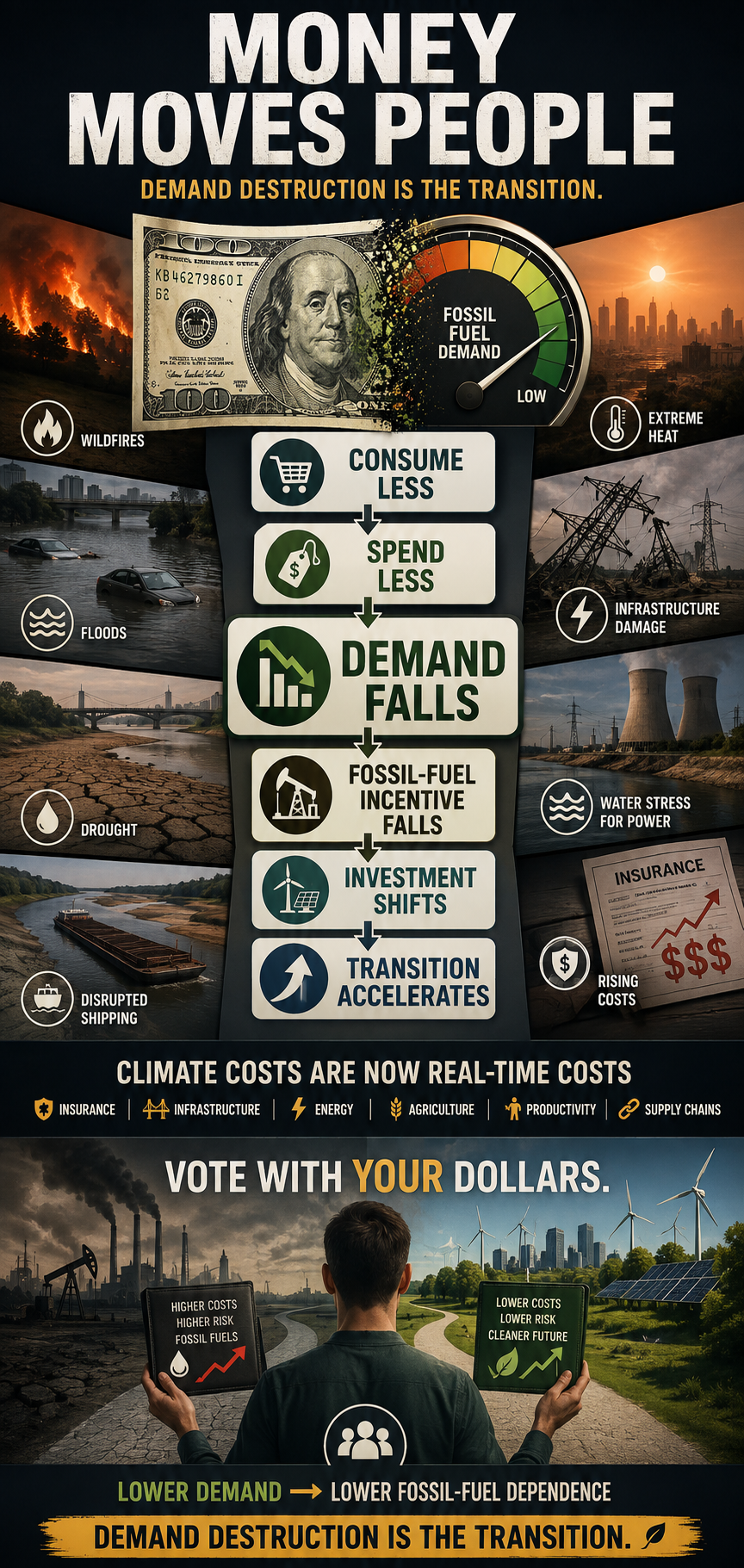
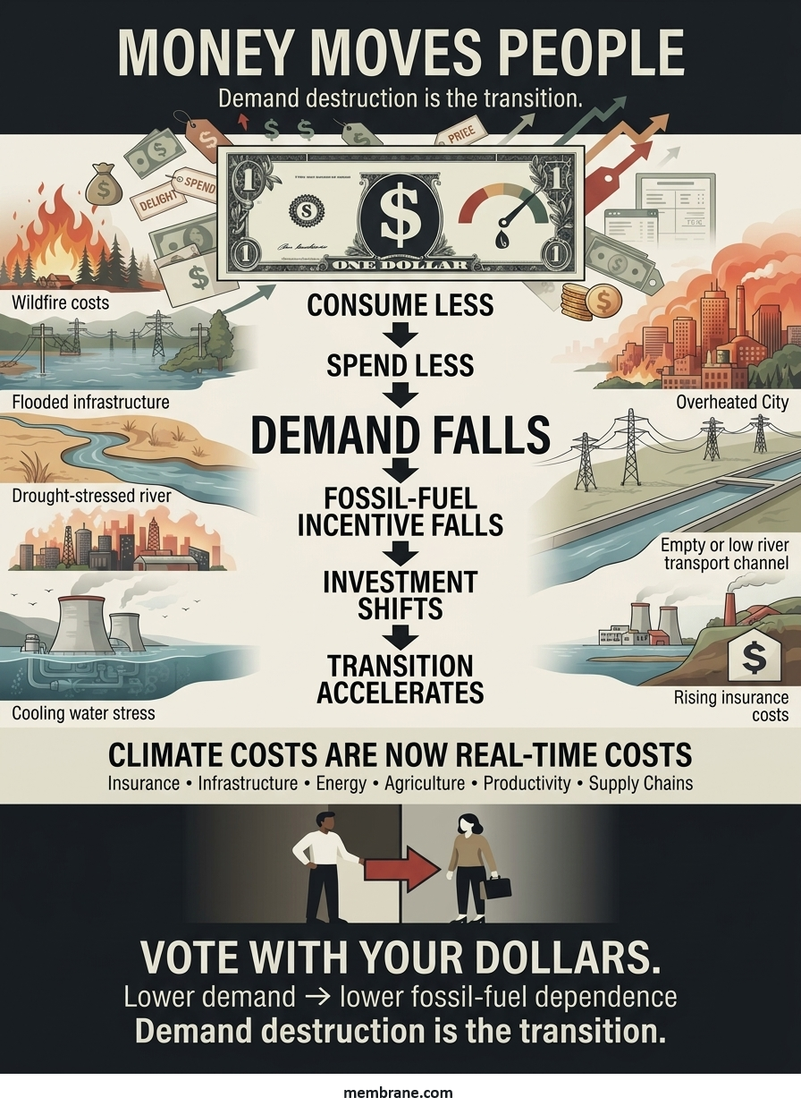
Consume less, and demand falls.

Demand falls, and the economic incentive to produce falls.

That is the mechanism.

The Economics of Personal Climate Stewardship

Today, only a small fraction of Americans appear to be pursuing a deliberately structured net-zero lifestyle through continuous behavioral reductions, efficiency improvements, and intentional balancing. But this does not mean the model cannot scale. The critical question is how climate stewardship is presented.

If reducing climate impact is framed exclusively as sacrifice, people resist. If it is framed as economic self-interest, the equation changes.

What happens when people discover that reducing unnecessary consumption can save them thousands of dollars a year?

What happens when energy efficiency lowers household expenses?

When smaller vehicles reduce fuel, maintenance, and insurance costs?

When reducing waste means buying fewer things that do not provide meaningful value?

When local production and durable goods become economically attractive?

When conservation becomes synonymous with financial resilience?

The behavior does not have to begin with ideology.

It can begin with a household budget.

Vote With Your Dollars

This is where the remaining majority of the population becomes economically important.

When millions of people begin making purchasing decisions based on cost, durability, efficiency, resilience, and environmental impact, they collectively alter demand.

When demand changes, markets respond. When fossil-fuel demand declines, the economic incentive to extract, refine, transport, and sell fossil fuels declines with it. This is fundamentally different from waiting for governments to impose every change from the top down. It is a bottom-up economic transition.

People do not have to agree about everything.

They do not have to become climate activists.

They do not even have to agree about climate policy.

They simply have to discover that some forms of consumption are no longer worth what they cost.

The Feedback Loop

The process can become self-reinforcing:

Lower unnecessary consumption
↓
Lower household costs
↓
Lower energy and resource demand
↓
Reduced fossil-fuel demand
↓
Lower economic incentive for fossil-fuel expansion
↓
Greater investment in alternatives and efficiency
↓
Further reductions in fossil-fuel demand

This is an economic feedback loop.

And unlike many climate-policy debates, it does not require everyone to agree on the destination before beginning the journey.

Demand Destruction Is the Transition

The transition away from fossil fuels is often described as a supply problem:

How quickly can we replace coal, oil, and natural gas?

But there is another side of the equation.

How quickly can we reduce the demand that makes fossil-fuel extraction profitable?

That may ultimately be the more powerful question.

We do not need to convince every person to become an environmentalist.

We need to make lower-carbon choices increasingly rational economic choices.

The climate crisis is already generating enormous costs. Insurance premiums are rising. Infrastructure is being stressed. Agricultural productivity is being disrupted. Heat is reducing labor capacity. Extreme weather is destroying capital. Supply chains are becoming more vulnerable.

These costs are not theoretical.

They are appearing on balance sheets, household budgets, insurance statements, government budgets, and corporate earnings reports.

The economic system is beginning to receive the bill.

And money moves people.

Demand destruction is not the enemy of the energy transition.

Demand destruction is the transition.

4.9% PPI: That’s Essentially 5% Producer Inflation

Posted on 2026/08/132026/08/13 by admin

by Daniel Brouse

A 4.9% year-over-year Producer Price Index (PPI) increase means the average price level producers face is nearly 5% higher than it was one year ago.

The math is straightforward:

5.0% − 4.9% = 0.1 percentage point

That puts the headline PPI rate just one-tenth of a percentage point below 5%.

For example, if an identical basket of wholesale goods cost a business $100,000 in July 2025, a 4.9% increase means that same basket would cost approximately $104,900 in July 2026.

And 4.9% doesn’t happen in isolation. Businesses are operating on a cost structure already elevated by previous years of inflation. The new increase compounds on top of those higher prices.

There is another important point: 4.9% is an average. Different industries can experience dramatically different increases. Businesses heavily dependent on energy, transportation, food, or raw materials can face considerably higher cost pressures.

Those higher producer costs can eventually move through the supply chain and put additional pressure on consumer prices.

So no, 4.9% isn’t technically 5.0%. But it is mathematically very close—and economically, a nearly 5% annual increase in producer prices is significant.

Do the math. Then look at what those numbers mean for the real economy.

The Oil Import Surge & Inventory Anomaly

While July wholesale energy costs fell and helped moderate the PPI data, the energy market itself is experiencing significant near-term turbulence amid the ongoing closure of the Strait of Hormuz and stalled U.S.-Iran negotiations.

This creates a bifurcated picture in the U.S. oil market: headline inventories are surging, but the increase appears to be driven primarily by an extraordinary jump in imports rather than a sudden expansion of domestic production.

• The Massive Build: The Energy Information Administration (EIA) reported a 17.4 million-barrel increase in U.S. commercial crude inventories for the week ending August 7. That was the largest single-week build since January 2023.

• The Import Catalyst: Net crude imports nearly doubled their recent four-week average, reaching approximately 4.28 million barrels per day. That surge points to an unusual compression in the commercial shipping and inventory cycle, with refiners sourcing substantially more crude from international markets.

• Refinery Strain: U.S. refinery utilization slipped only 0.3 percentage points to 96.2%. That remains an extremely high utilization rate and suggests refiners are operating near capacity while the market adjusts to disrupted international supply routes.

The important distinction is this: A massive inventory build does not automatically mean the underlying oil market is oversupplied.

In this case, the inventory increase appears closely tied to an extraordinary surge in imports and the disruption of normal shipping patterns. The numbers therefore need to be interpreted within the broader geopolitical and logistical environment.

The headline inventory number tells only part of the story. The flow of crude into the country—and why that flow changed so dramatically—is the more important signal.

“According to newly released data from GasBuddy and the American Automobile Association (AAA), the national average price of gasoline has never been above $4.00 a gallon this late in the calendar year.“

July 2026: The Record Heat Was Especially Dangerous After Sunset

Posted on 2026/08/12 by admin

by Daniel Brouse

July 2026 was officially the hottest month ever recorded for the contiguous United States since national records began in 1895. According to the National Oceanic and Atmospheric Administration (NOAA), the average temperature across the Lower 48 reached 76.9°F—about 3.3°F above the 20th-century average and roughly 0.1–0.2°F warmer than the previous July records set during the Dust Bowl era in 1936 and the exceptional heat of 2012.

But the most important part of this record may not have been the daytime heat.

It was the heat that refused to leave at night.

The nighttime record is the real warning signal

July’s average daytime maximum temperature was 89.5°F, which was 2.9°F above average and ranked as the sixth-warmest month on record for average high temperatures.

The average overnight minimum temperature, however, reached 64.2°F—an extraordinary 3.7°F above average. That was the warmest average minimum temperature ever recorded for the contiguous United States, surpassing the previous record, set in July 2022, by 0.7°F.

That distinction matters.

A hot afternoon is dangerous, but a hot afternoon followed by a substantial nighttime cooldown gives the human body, vegetation, soils, buildings, infrastructure, and electrical systems an opportunity to recover.

When nighttime temperatures remain elevated, that recovery period disappears.

July 2026 therefore represents more than another record for daytime heat. It demonstrates an increasingly important characteristic of a warming climate: the thermal baseline is rising around the clock.

Why nighttime temperatures matter so much

Nighttime cooling is a fundamental part of Earth’s daily heat cycle.

After sunset, the land surface normally loses energy through infrared radiation. As the surface cools, the air near the ground cools as well. This produces the familiar drop from afternoon highs to early-morning lows.

Greenhouse-gas-driven warming interferes with that process. A warmer atmosphere contains more heat and can emit more infrared radiation back toward the surface. Increased atmospheric moisture can further enhance this effect because water vapor is itself a powerful greenhouse gas.

Cloud cover, humidity, soil moisture, wind, urbanization, and atmospheric circulation also influence how much the temperature falls overnight.

The result is not simply that afternoons become hotter. The floor beneath the temperature curve rises. That is critically important because the minimum temperature determines how much accumulated heat is actually released before the next day begins. If an afternoon reaches 100°F but the temperature falls to 65°F overnight, the body and environment experience a meaningful period of relief. If that same afternoon is followed by an 82°F night, the next day begins with the system already carrying a substantial heat load.

This is why nighttime warming can transform an episodic heatwave into a cumulative heat event.

The human body needs nighttime recovery

The human body is particularly vulnerable to persistent nighttime heat because sleep is one of the primary periods available for physiological recovery.

During sleep, the body normally reduces its core temperature. A hot bedroom makes that process more difficult. Higher nighttime temperatures can increase sweating, heart rate, dehydration, and thermal stress while disrupting normal sleep.

Research examining hundreds of thousands of U.S. respondents found that increases in nighttime temperatures were associated with more reports of insufficient sleep, with particularly strong effects during summer.

The consequences extend beyond simply feeling tired the next morning.

Repeated nights of inadequate sleep can impair cognitive performance, mood, immune function, metabolic regulation, and the ability to cope with additional heat stress.

Nighttime heat therefore creates a potentially dangerous cycle:

Hot day → inadequate nighttime cooling → poor sleep and incomplete recovery → greater vulnerability the next day → another hot day.

Research specifically examining nighttime warming has also found significant associations between hot nights and mortality. One modeling study concluded that nighttime warming could become an increasingly important component of future heat-related mortality, with the mortality risk on hot nights substantially higher than on days without hot nighttime conditions.

More recent multicountry research likewise finds that hot nights themselves contribute independently to heat-related mortality risk.

In other words, nighttime heat is not merely an inconvenience between two hot days. It is itself a health hazard.

The agricultural implications are equally important

Plants do not stop metabolizing when the sun goes down.

At night, plants continue to respire. They consume stored energy and undergo physiological processes that are essential for growth, reproduction, and recovery from daytime stress. When nighttime temperatures remain unusually high, respiration increases and plants can consume more of the carbohydrates they produced during the day.

Research involving wheat has demonstrated this effect experimentally. A field study found that artificially increasing nighttime temperatures by 2°C reduced grain yield, with yield declining by approximately 1.9% for every 1°C increase in nighttime temperature in the experiment.This is especially significant because nighttime warming can affect crops even when daytime temperatures do not become dramatically more extreme.

A crop can therefore experience a double burden:

More daytime heat stress + less nighttime physiological recovery.

Higher nighttime temperatures can also increase water loss and alter plant stomatal behavior, while warmer soils can accelerate moisture loss and biological activity. For agriculture, the problem is not simply the temperature at noon. It is the accumulated thermal stress across the entire 24-hour cycle.

Nighttime heat also keeps the landscape from resetting

The same principle applies beyond human beings and crops.

Soils need to cool.

Water bodies need to release heat.

Buildings need to dissipate stored heat.

Urban infrastructure needs to shed the energy accumulated during the day.

Even ecosystems depend upon daily temperature cycles.

When nights remain warm, all of these systems begin the following day from a higher thermal starting point.

This can become particularly important during prolonged heatwaves. Consider two hypothetical heatwaves with identical daytime highs:

Heatwave A:
100°F day → 65°F night → 100°F day → 65°F night

Heatwave B:
100°F day → 82°F night → 100°F day → 82°F night

The daytime maximum is identical.

But Heatwave B is vastly more difficult for people, plants, buildings, soils, and ecosystems because the system never receives the same opportunity to cool.

That is the hidden dimension of persistent heat.

Nighttime warming can amplify the consequences of daytime warming

It is important to be precise here: rising nighttime temperatures should not be described as a standalone climate “feedback” in the strict physical sense. Rather, nighttime warming is both a consequence of increased heat retention in the climate system and an amplifier of the impacts produced by daytime warming.

The distinction matters.

The physical climate system contains genuine feedbacks—such as increased atmospheric water vapor, declining snow and ice, and changes in soil moisture—that can amplify warming.

Nighttime warming is an important expression of those processes at the surface.

And once it occurs, it can amplify consequences across other systems.

For example:

Higher greenhouse-gas concentrations → greater atmospheric heat retention → warmer nights → less nighttime recovery → greater human heat stress → greater vulnerability to the next day’s heat.

A parallel agricultural pathway is:

Warmer nights → increased plant respiration and physiological stress → reduced recovery → lower productivity → greater vulnerability to subsequent heat and drought.

This is why minimum temperatures deserve far more attention than they traditionally receive.

The energy system feels it too

There is another important consequence: electricity demand.

Hot afternoons increase air-conditioning demand. But when temperatures remain high overnight, air conditioners continue operating long after sunset.

That extends the period of peak or elevated electricity demand and reduces the opportunity for buildings to naturally cool.

Instead of a system experiencing:

high demand → nighttime relief → recovery

the grid can experience:

high demand → continued overnight demand → high demand again.

This becomes especially problematic when multiple consecutive days and nights are exceptionally warm.

The result is a compound infrastructure stress rather than a single afternoon peak.

Nighttime temperatures reveal accumulated heat

There is also a deeper climate signal embedded in minimum temperatures.

Daytime temperatures can be strongly influenced by short-term weather conditions, including sunshine, wind, soil moisture, and atmospheric circulation. Minimum temperatures are also affected by these factors, but persistently elevated nighttime temperatures can reveal something particularly important: the atmosphere and surface are retaining more heat between sunset and sunrise.

That makes nighttime minimums an important indicator of how the climate system is changing.

July 2026 provides an extraordinary example.

The United States did not merely experience exceptionally hot afternoons.

It experienced exceptionally warm mornings.

The average minimum temperature was 3.7°F above normal—an even larger anomaly than the daytime maximum—and established a national record by a substantial margin.

That is why the July 2026 record deserves to be examined differently from a conventional heat record.

The most important number may be 64.2°F, not 89.5°F.

A warmer baseline changes what “extreme” means

There is another consequence that is easy to overlook.

As nighttime temperatures rise, the definition of a dangerous heat event changes.

Historically, a very hot day followed by a relatively cool night allowed the human body and natural systems to partially recover. But as the nighttime baseline rises, temperatures that once represented nighttime relief can themselves become hazardous.

The result is a compression of the daily thermal cycle.

The difference between daytime and nighttime temperatures becomes smaller, while the entire 24-hour temperature profile shifts upward. This means climate change is not simply producing more extreme peaks. It is elevating the entire thermal floor.

And once that floor rises sufficiently, heat becomes persistent rather than episodic.

July 2026 fits into a larger global pattern

The U.S. record occurred within an exceptionally warm global month. According to the Copernicus Climate Change Service, July 2026 was the joint-second-warmest July globally, tied with July 2024. Global ocean surface temperatures outside the polar regions were the highest recorded for any July, with developing El Niño conditions contributing to the unusually warm ocean state.

NOAA also reports that El Niño is continuing to strengthen and is expected to persist into early 2027, adding another natural source of variability to an already substantially warmer climate background.

El Niño can help explain why a particular period becomes exceptionally warm, but it does not explain away the long-term warming trend. Natural variability operates on top of a climate system whose baseline has been shifted upward by human-caused greenhouse-gas emissions.

That distinction is essential.

The warning hidden in the overnight record

July 2026 should therefore not be remembered simply as the month when the United States broke another temperature record. It should be remembered as a month when the nighttime thermal floor rose dramatically. The record daytime heat was dangerous. The record nighttime heat made it harder to recover from that danger.

For people, that means poorer sleep and greater cumulative heat stress. For agriculture, it means less nighttime recovery and additional physiological stress. For buildings and power systems, it means less overnight cooling and prolonged energy demand. For soils and ecosystems, it means less opportunity to shed accumulated heat.

And for the climate system itself, it is another indication that the traditional rhythm of hot day → cool night → recovery is being disrupted.

That is the significance of rising nighttime temperatures.

A hotter afternoon creates heat stress. A hotter night prevents the system from recovering from it.

When both happen repeatedly, heat stops behaving like a series of isolated events and begins behaving like a persistent environmental load.

That may ultimately be one of the most consequential—and least appreciated—features of a warming climate.

Integrated Climate Stewardship: The Fossil Fuel Question and Answer

Posted on 2026/08/112026/08/11 by admin

Question:

I use phasing out in a way that means completely ending the use and production of fossil fuels down to zero. Phasing down means a gradual reduction or scaling back in FF use over time without specifying a complete stop. Would add or alter that in any way?

How would you define differntiate ‘transition away’?

Reply:

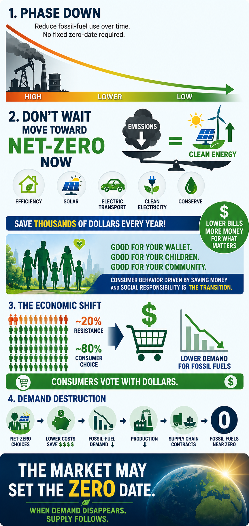
I would slightly modify your definition of “phasing down” to: “a gradual reduction or scaling back in fossil-fuel use over time without specifying a date for complete cessation.”

There are really two separate issues for me:

1. For this generation, I prefer net-zero carbon emissions as the immediate goal. If someone isn’t already moving toward net-zero, I think they should start now. We don’t need to wait for a theoretical future phase-out date to begin reducing emissions.

2. As both a climatologist and an economist, I’m not convinced that setting a specific date for the complete elimination of fossil fuels is ultimately what matters. In the U.S., roughly 20% of the population appears ideologically committed to policies that would accelerate climate change. Nothing I say or do is likely to change that.

But that still leaves roughly 80% of the population—and I think economics is going to do much of the work.

Right now, perhaps only ~0.5% of Americans are seriously attempting a structured net-zero lifestyle through continuous behavioral reductions and intentional balancing. As more people discover that net-zero can actually save them thousands of dollars a year while also leaving a better environment for their children and grandchildren, I expect consumer behavior to change.

When the remaining ~79.5% begin voting with their dollars, fossil-fuel demand will fall. That creates demand destruction, which ultimately means suppliers will have less and less reason to produce fossil fuels.

So, ironically, I don’t think we necessarily need to establish the exact date when fossil fuels reach zero. The market may establish that date for us. The “complete stop” happens when there is no longer sufficient demand to sustain the fossil-fuel supply chain.

Question:

When you use the term net zero is it with the understanding that the “net” component allows continuous greenhouse gas emissions under the assumption that unproven removal technologies or flawed offsets will balance them out later, delaying necessary fossil fuel phaseouts?

Net zero is a contentious term within my community and I want to be clear that I understand how you see and apply it.

Reply:

That’s an important distinction. When I use the term net-zero, I’m talking about it at the personal/lifestyle level, and I am not using “net” to justify continuing to emit greenhouse gases while assuming that unproven technologies or questionable offsets will clean up the problem later.

What I mean is closer to “Holistic Net-Zero Living” or “Integrated Climate Stewardship”: reducing and, wherever realistically possible, zeroing out the emissions associated with my own lifestyle first, while also taking responsibility for the impacts I can’t immediately eliminate.

For me, that means a 360-degree carbon strategy:

ZEROING OUT / STRUCTURAL DECARBONIZATION

Electrifying transportation and home energy
Increasing energy efficiency
Using clean electricity
Reducing fossil-fuel consumption as close to zero as practical
Reducing high-carbon consumption, including dietary choices

BEYOND MY DIRECT FOOTPRINT

Supporting ecosystem restoration and conservation
Protecting forests and biodiversity
Supporting businesses and technologies that accelerate decarbonization
Using my purchasing and investment decisions to create economic demand for cleaner alternatives

So I’m not saying, “Keep emitting and someone will remove it later.” Quite the opposite. The first priority is eliminating the emissions themselves.

I think of the “net” component as recognizing that an individual cannot instantly eliminate every indirect emission associated with modern life. Rather than pretending those emissions don’t exist, I try to compensate through additional positive actions while continuously working to reduce the underlying footprint.

Ultimately, my goal isn’t simply to achieve a favorable carbon-accounting number. It’s to change the way I live so that my actual fossil-fuel demand approaches zero—and to use my economic choices to help make that transition happen systemically.

That’s why I sometimes think “holistic net-zero living” or “integrated climate stewardship” communicates what I mean better than simply saying “net-zero.”

Question:

Why continue using the language of ‘net zero’? What economic model do you see best aligns w/ what you have outlined?

Reply:

Haaha… good questions.

A: I’m actually in the process of writing the paper that officially changes my language from “net-zero” to “Integrated Climate Stewardship.” So thank you for pushing me on that. I think the new terminology better captures what I’ve been trying to describe.

B: I’m also working on the economic model, and that one is considerably trickier—not because of the terminology, but because AI is changing the underlying economics so rapidly.

I see AI as a double-edged sword. On one edge, as AI replaces more human labor and productivity, the human contribution to economic production could eventually become a much smaller share of GDP. AI may also be capable of producing enormous amounts of economic value with far less energy per unit of output than traditional human labor and many existing production systems.

But the other edge of that sword is wealth distribution.

If the ownership of AI, capital, and productive capacity becomes increasingly concentrated, we could see extraordinary productivity growth occurring alongside increasingly unjust wealth inequality. We could potentially solve one problem—resource and energy efficiency—while creating another: who actually owns and benefits from the productivity?

That’s the economic model I’m wrestling with now: how do we build an economy where AI-driven productivity, decarbonization, consumer savings, and environmental stewardship reinforce each other while the resulting wealth is broadly distributed?

That may ultimately be a much bigger economic question than the climate transition itself.

Question:

Have you been sitting with the economic of degrowth in all of this then? Sounds like there is that tension in what is being considered.

Reply:

Yes. I’ve been sitting with the economics of degrowth quite a bit. And I think there’s an interesting tension here.

Traditional capitalism is fundamentally tied to population growth, human labor, productivity, and consumption. But AI potentially breaks that relationship. If technology increasingly replaces human labor, then economic growth can continue—even accelerate—while the economic value of human labor declines, perhaps dramatically.

So I’m not sure the future necessarily looks like “degrowth.” It may be something stranger: exponential technological growth occurring alongside declining human labor demand, an aging population in the developed regions of the world, and potentially declining population worldwide.

That raises a much bigger question: if human labor is no longer the primary engine of economic value, what exactly are we trying to maximize—and how should the economy distribute the benefits of that productivity?

That’s the economic model I’m wrestling with right now.

Question:

What about lands and waters in these considerations?

Can we agree that what we need must be either mined or grown?

Raw materials come from somewhere with significant externalities — often left out of economic theory.

My other issue is the assumptive ghost of interest-bearing-debt as a driver of unnecessary growth.

Reply:

Yes—and I think land, water, and raw materials have to be part of the model. My initial modeling, however, is pointing toward a very different problem than the one we traditionally assume.

If AI continues improving itself, productivity could eventually become extraordinarily resource-efficient. Very little additional human labor—and potentially much less land, water, or energy per unit of economic output—may be required for productivity and growth. At the same time, consumers could be forced to consume much less because their income from labor is declining. And as solar and other clean-energy technologies continue becoming cheaper, the pressure for some forms of mining and extraction could decline as well.

That brings me back to your point about interest-bearing debt. I think sovereign debt may become the critical part of the equation.

Productivity gains and abundant cheap clean energy are profoundly deflationary. Deflation sounds wonderful for consumers in theory—but not if it is accompanied by collapsing labor income. You could have falling costs and prices while households simultaneously lose the purchasing power needed to buy anything.

Now add governments facing enormous debt obligations while their traditional tax base is shrinking because human labor is becoming less economically valuable. Governments could increasingly rely on interest-bearing debt to finance poverty reduction, redistribution, and some form of basic income.

And that creates a potentially nasty feedback loop: AI-driven productivity → declining labor income → shrinking tax base → rising sovereign debt → greater reliance on monetary expansion → inflationary pressure.

Historically, severe sovereign debt problems have sometimes been resolved through substantial currency devaluation and inflation. I’m not saying hyperinflation is inevitable—but it is one of the risks I’m now modeling.

The really strange possibility is that we could simultaneously have exponential productivity, increasingly abundant cheap energy, falling costs of production—and increasing economic hardship for ordinary people.

In other words, the problem may not ultimately be whether the planet can produce enough. It may be whether humans can maintain enough income, purchasing power, and economic agency to participate in the abundance that AI creates.

That, to me, is where the economic model gets really interesting.