“The greater risk is a gradual degradation of living standards if adaptation is delayed.“
by Daniel Brouse
Introduction
Climate change is often discussed as if it will either produce an imminent societal collapse or, conversely, have little economic consequence. Neither view is supported by the physical science.
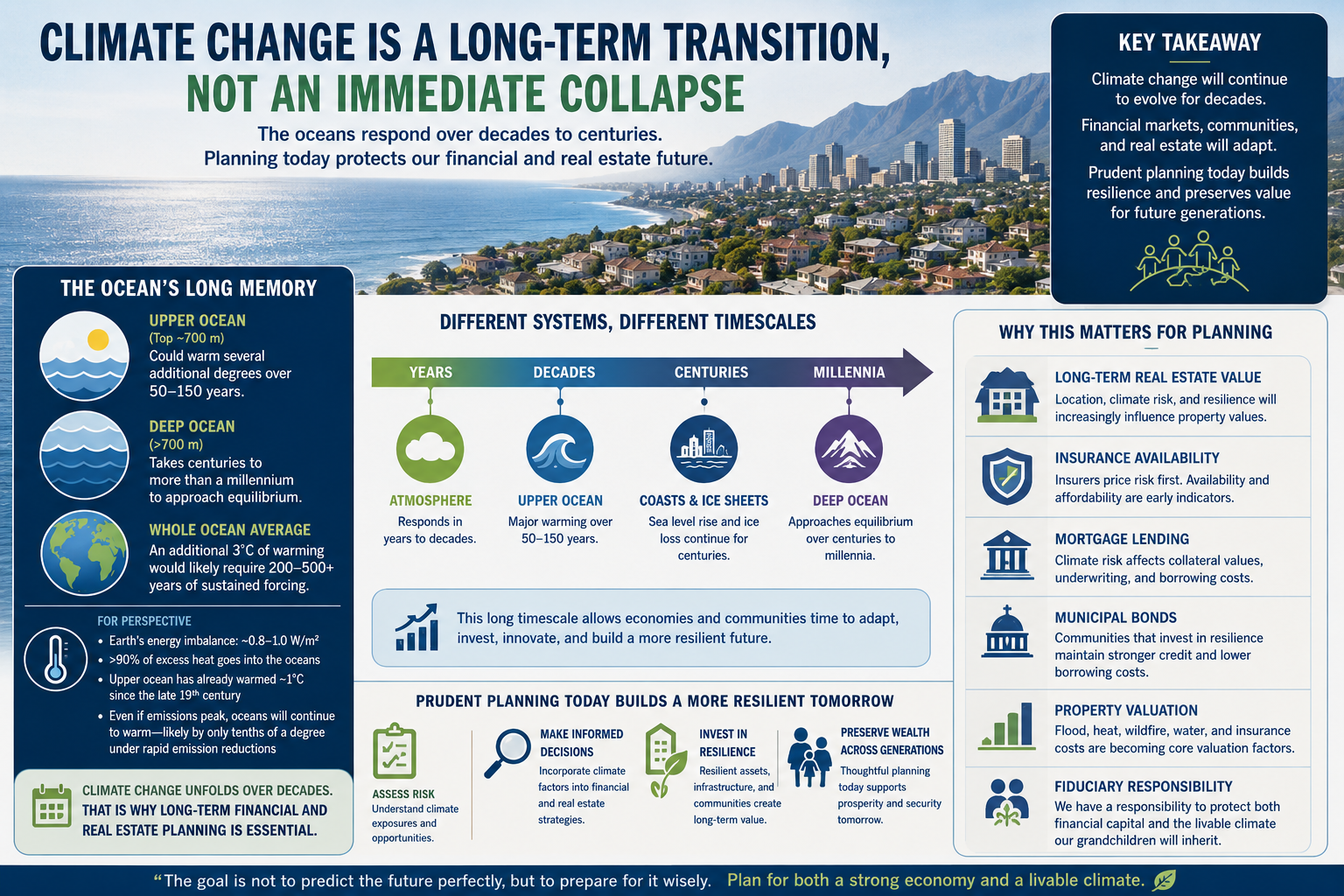
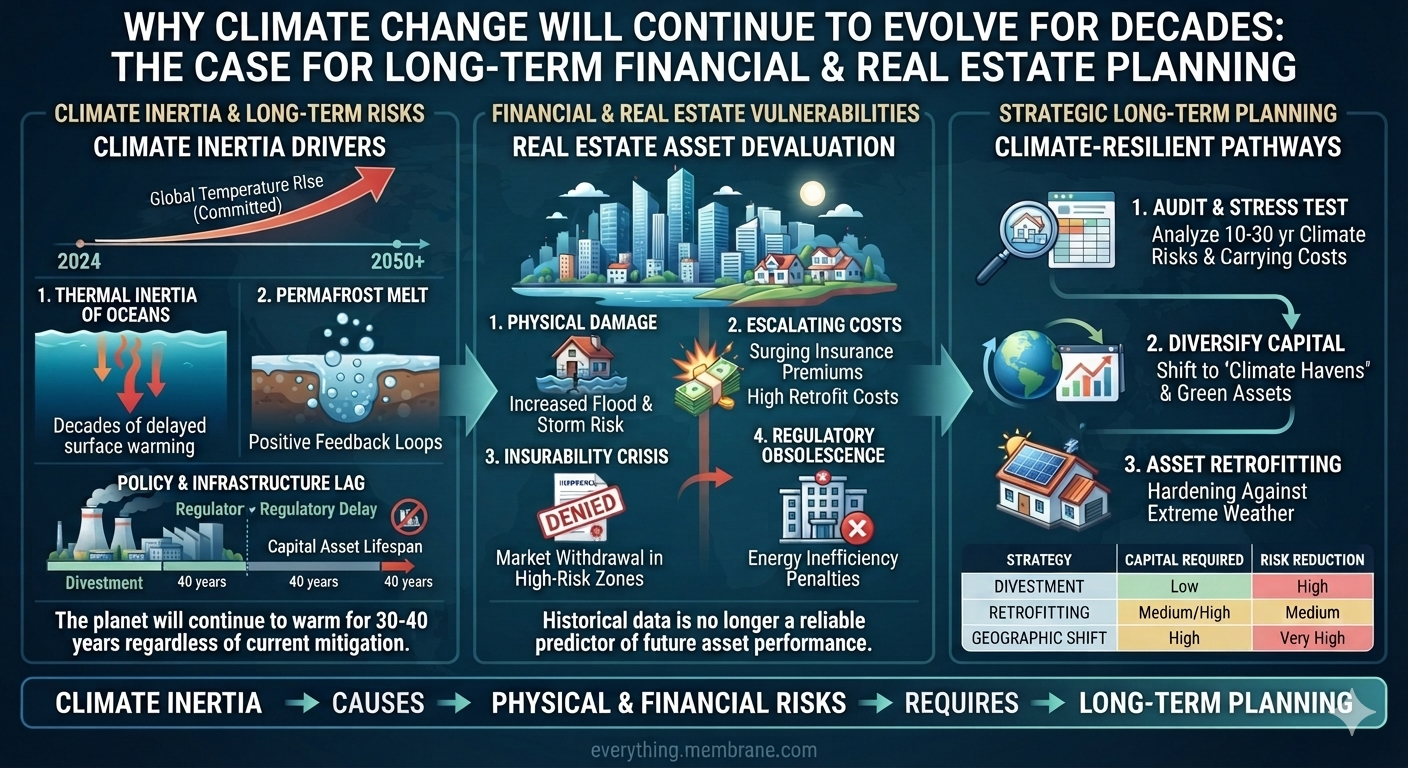
The Earth’s climate system responds over multiple timescales. While the atmosphere reacts relatively quickly to changes in greenhouse gas concentrations, the oceans—the planet’s largest heat reservoir—respond much more slowly. This difference, known as thermal inertia, means that many of the economic consequences of climate change will continue to unfold over decades, regardless of whether emissions peak today or several years from now.
For investors, homeowners, businesses, insurers, lenders, and governments, this distinction is critical. The evidence points not toward an immediate collapse of the global economy, but toward a long period of increasing environmental risks that will progressively reshape financial markets and real estate values.
The Ocean’s Long Memory
If greenhouse gas concentrations remained near current levels long enough to maintain today’s radiative forcing, it would likely take many decades to centuries for the global ocean to warm by an additional 3°C.
Current scientific understanding suggests:
The upper ocean (roughly the top 700 meters) could warm several additional degrees over approximately 50–150 years.
The deep ocean requires centuries to more than a millennium to approach equilibrium.
The global ocean average would likely require several centuries of sustained forcing to warm another 3°C.
More than 90% of Earth’s excess heat enters the oceans, giving the climate system enormous momentum.
Even if atmospheric temperatures stabilize, sea level rise, marine heat waves, glacier retreat, and many coastal impacts continue because the oceans continue redistributing heat.
Climate change therefore behaves less like flipping a switch and more like steering an aircraft carrier. Once underway, changes continue for decades.
Why This Does Not Mean Immediate Economic Collapse
The nonlinear acceleration of climate change does not imply that modern economies disappear within a few years.
Economic systems continually adapt.
History demonstrates remarkable resilience through world wars, financial crises, pandemics, technological revolutions, and natural disasters. Markets evolve. Capital reallocates. Infrastructure is rebuilt. New technologies emerge.
Climate change represents another major structural transformation—not an instantaneous end to economic activity.
The greater risk is a gradual degradation of living standards if adaptation is delayed.
Financial Markets Price Risk—They Do Not Ignore It
Climate risk is becoming another measurable input.
Rather than causing markets to cease functioning, climate change increasingly changes how capital is allocated.
Investment flows are likely to favor:
Resilient infrastructure
Water management
Energy efficiency
Distributed power systems
Climate-resilient agriculture
Advanced building technologies
Adaptation engineering
Markets rarely stop functioning.
They reprice risk.
Mortgage Lending in a Changing Climate
Mortgage lending has always depended upon one fundamental assumption:
The collateral will retain value over the life of the loan.
Most residential mortgages extend 15 to 30 years.
Commercial financing often spans decades.
Those time horizons now overlap directly with accelerating climate risks.
Lenders are increasingly evaluating:
Flood exposure
Wildfire probability
Coastal erosion
Extreme heat
Water availability
Infrastructure resilience
Local adaptation policies
Climate risk is becoming credit risk.
Properties with increasing exposure may experience:
Higher insurance costs
Larger reserve requirements
Lower loan-to-value ratios
Increased underwriting scrutiny
Higher borrowing costs
Conversely, resilient communities with strong infrastructure may receive more favorable financing because they present lower long-term risk.
Climate-informed lending is simply modern risk management.
Insurance Availability May Become the First Market Signal
Insurance companies often detect climate risk before property markets do.
Unlike homeowners, insurers continuously update catastrophe models using the latest observations and loss data.
When risks increase, insurers respond by:
Raising premiums
Increasing deductibles
Restricting coverage
Reducing policy limits
Withdrawing from selected markets
Recent developments in wildfire-prone states, hurricane-exposed coastlines, and hail-prone regions illustrate this trend.
In many communities, insurance affordability—not property damage itself—may become the first significant economic consequence of climate change.
Without affordable insurance:
Mortgage financing becomes more difficult.
Homeownership becomes more expensive.
Property values may weaken.
Municipal tax bases can come under pressure.
Insurance increasingly serves as an early warning system for long-term climate risk.
Municipal Bonds and Local Government Finance
Climate resilience is increasingly becoming a municipal finance issue.
Cities and counties finance much of their infrastructure through municipal bonds.
Those bonds ultimately depend upon:
Stable tax revenues
Economic growth
Reliable infrastructure
Sustainable operating costs
As climate risks increase, municipalities may require additional investments in:
Flood control
Stormwater systems
Water supply
Cooling infrastructure
Grid modernization
Emergency services
Road and bridge resilience
Communities that invest proactively may maintain stronger credit quality over time.
Communities that defer adaptation could face rising maintenance costs, increasing insurance expenses, and pressure on their fiscal health.
For municipal investors, climate resilience increasingly becomes part of long-term credit analysis.
Property Valuation Is Becoming Dynamic
Historically, property valuation focused on:
Location
Schools
Transportation
Employment
Neighborhood quality
Climate is becoming another location characteristic.
Future valuation models will likely incorporate increasing amounts of climate-related information, including:
FEMA flood maps
Local flood history
Heat exposure
Wind risk
Wildfire potential
Water reliability
Insurance costs
Building resilience
Community adaptation investments
Properties will not simply gain or lose value because of climate change.
Rather, markets will increasingly differentiate between properties based on their long-term resilience.
The result is likely to be greater divergence between communities that prepare and those that do not.
Investment Implications
Because climate impacts unfold over decades, financial planning becomes more—not less—important.
Assuming there will be “no economy” several years from now is neither supported by economic history nor by climate science.
Instead, investors should recognize that long-term wealth preservation increasingly depends upon understanding long-term environmental risk.
That includes:
Diversified investment portfolios.
Climate-informed real estate decisions.
Appropriate insurance coverage.
Infrastructure resilience.
Geographic diversification.
Long-term retirement planning.
Planning remains one of the strongest tools available for reducing future financial risk.
Fiduciary Responsibility Across Generations
Every generation inherits assets built by those before it.
Likewise, every generation passes assets forward.
That fiduciary responsibility extends beyond investment portfolios.
It includes:
Homes.
Communities.
Infrastructure.
Businesses.
Natural resources.
Financial systems.
Protecting both environmental and financial capital is not a contradiction.
It is prudent stewardship.
Planning for climate risk is no different than planning for inflation, demographic change, technological disruption, or changing interest rates.
Responsible investors prepare for foreseeable risks rather than assuming those risks either do not exist or will immediately end the economic system.
Conclusion
Climate science indicates that many impacts will continue evolving over decades because Earth’s oceans absorb and release heat slowly.
That long timescale does not support predictions of imminent economic collapse.
Instead, it points toward an extended period during which markets continuously adapt by repricing risk, directing capital toward resilience, and rewarding long-term planning.
For homeowners, investors, lenders, insurers, businesses, and governments, the challenge is not deciding whether there will be an economy.
The challenge is helping shape an economy that is both financially resilient and environmentally sustainable.
The goal is not simply to leave future generations a larger investment portfolio.
It is to leave them both a livable climate and an economy capable of supporting opportunity for decades to come.
Straight-line winds are among the most destructive weather hazards on Earth, yet they often receive far less public attention than tornadoes and hurricanes. These powerful, non-rotational winds can flatten forests, rip roofs from buildings, topple power lines, and cause widespread infrastructure failures. In many cases, the damage resembles the aftermath of a tornado or even a hurricane.
Unlike tornadoes, which concentrate damage within a rotating vortex, straight-line winds can devastate broad regions simultaneously. Wind speeds frequently exceed 70–100 mph and, in extreme cases, may surpass 140 mph. Because they can strike with little warning and affect large geographic areas, straight-line wind events represent a growing hazard to communities, transportation systems, utilities, and the insurance industry.
Emerging research indicates that climate change is altering the atmospheric ingredients that produce severe convective storms. As the atmosphere warms and stores more energy, straight-line wind events are becoming more frequent, more destructive, and increasingly widespread. These changes are transforming severe convective storms into one of the fastest-growing sources of weather-related economic losses in the United States.
What Are Straight-Line Winds?
Straight-line winds are powerful horizontal winds that move outward from their source without rotating. They are most commonly produced by the downward plunge and subsequent outward surge of rain-cooled air from severe thunderstorms.
Unlike tornadoes, which draw air inward and rotate violently around a central vortex, straight-line winds push air exclusively outward along the ground. Despite this difference, their destructive potential can rival or even exceed that of weak-to-moderate tornadoes.
The Lifecycle of a Straight-Line Wind Event
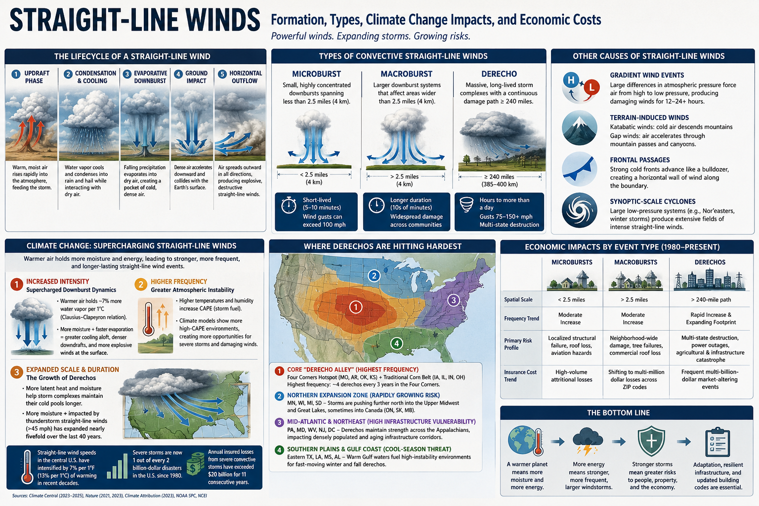
1. Updraft Phase
Warm, moist air rises rapidly into the atmosphere, feeding the development of a growing thunderstorm.
2. Condensation and Cooling
As water vapor ascends, it cools and condenses into rain and hail while interacting with surrounding layers of drier air.
3. Evaporative Downburst Formation
Falling precipitation evaporates into dry air aloft. Because evaporation absorbs heat, it creates a large pocket of extremely cold, dense air.
4. Ground Impact
This dense air mass accelerates downward as a powerful downdraft and collides with Earth’s surface.
5. Horizontal Outflow
Upon impact, the descending air can no longer move downward. Instead, it compresses and surges outward in all directions, producing an explosive burst of destructive straight-line winds.
Classification of Convective Straight-Line Wind Events
Meteorologists classify thunderstorm-generated straight-line winds according to their size and duration.
Microbursts
Microbursts are highly concentrated downbursts spanning less than 2.5 miles (4 km). Although typically lasting only five to ten minutes, they can produce sudden wind gusts exceeding 100 mph and are particularly dangerous because of their intensity and lack of warning.
Macrobursts
Macrobursts are larger downburst systems that spread destruction across areas wider than 2.5 miles (4 km) and often persist significantly longer than microbursts.
Derechos
Derechos are massive, long-lived convective storm systems that produce continuous swaths of wind damage extending at least 240–250 miles (385–400 km). By definition, derechos generate sustained winds of at least 58 mph, with gusts commonly ranging between 75 and 150 mph.
Other Causes of Straight-Line Winds
Although convective downbursts are the most common source of straight-line winds, meteorologists classify any non-rotational horizontal wind as a straight-line wind, regardless of its origin.
Gradient Wind Events
These winds arise from large differences in atmospheric pressure. Air naturally flows from areas of high pressure toward low pressure. When powerful pressure systems are positioned close together, the resulting pressure gradient can accelerate air to damaging speeds. Unlike thunderstorm downbursts that last only minutes, gradient wind events can persist for 12 to 24 hours or longer.
Terrain-Induced Winds
Mountain landscapes frequently create severe straight-line winds.
Katabatic Winds: Cold, dense air descends from elevated plateaus or ice sheets under the influence of gravity, accelerating dramatically before spreading across valleys below.
Examples include:
Santa Ana winds in California
Bora winds in southeastern Europe
Gap Winds: Air masses forced through narrow mountain passes and canyons become compressed and accelerated, producing intense horizontal wind speeds.
Frontal Passages
The leading edge of a strong cold front can generate destructive straight-line winds. As dense cold air advances, it acts like an atmospheric bulldozer, forcing warmer air upward and creating a powerful wall of horizontal wind along the frontal boundary.
Synoptic-Scale Extratropical Cyclones
Large non-tropical low-pressure systems, such as Nor’easters and major winter storms, produce extensive fields of intense straight-line winds through tightly packed pressure gradients extending across hundreds of miles.
Climate Change and the Intensification of Straight-Line Winds
Climate change directly influences the atmospheric variables that fuel severe convective storms, causing thunderstorm-generated straight-line winds to become more frequent, intensely destructive, and geographically expanded.
Research synthesized by Climate Central and peer-reviewed studies published in Nature indicates that straight-line wind speeds across portions of the central United States have already intensified by approximately 7% per 1°F (13% per 1°C) of atmospheric warming during recent decades.
Several physical mechanisms are driving these changes.
The fundamental engine behind a straight-line wind event is the evaporative downburst. Climate change amplifies this process in multiple ways.
Higher Atmospheric Moisture Capacity
According to the Clausius-Clapeyron relationship, a warmer atmosphere can hold approximately 7% more water vapor for every 1°C increase in temperature. This additional moisture allows thunderstorms to contain substantially greater amounts of precipitation.
Enhanced Evaporative Cooling
When this larger volume of precipitation falls through relatively dry layers of air, evaporation occurs more rapidly. The evaporation dramatically cools the descending air, making it denser and heavier than its surroundings.
The greater the temperature contrast between the chilled downdraft and the surrounding environment, the faster the air accelerates downward. The result is a more violent impact at the surface and stronger, more destructive straight-line wind speeds.
Severe convective storms require highly unstable atmospheric conditions.
Elevated Convective Available Potential Energy (CAPE)
Warmer temperatures and increased humidity elevate Convective Available Potential Energy (CAPE), a measure of the energy available for thunderstorm development.
More Severe Storm Environments
Advanced climate models consistently project increases in high-CAPE environments under continued greenhouse gas forcing. These environments provide more opportunities for ordinary thunderstorms to intensify into severe systems capable of producing damaging straight-line winds.
3. Expanded Scale and Duration: The Growth of Derechos
Climate change also appears to be altering the longevity and geographic footprint of large convective systems.
Longer-Lived Storm Complexes
A warmer atmosphere contains greater amounts of latent heat and moisture, enabling storm systems to maintain their rain-cooled cold pools for longer periods. Because these cold pools drive storm propagation, straight-line wind events can persist over hundreds of miles.
Fivefold Geographic Expansion
Research summarized by Climate Attribution indicates that the total area affected by thunderstorm-generated straight-line winds exceeding 45 mph has expanded nearly fivefold during the past forty years. Regions farther north and east that historically experienced fewer severe wind events are increasingly experiencing high-intensity derecho systems.
The Severe Convective Storm Crisis
The financial consequences of straight-line winds have fundamentally changed since 1980. Driven by climate change, expanding development patterns, and inflation, severe convective storms have become the most frequent billion-dollar disaster category in the United States.
According to Climate Central, severe storms now account for approximately one out of every two billion-dollar weather disasters recorded since 1980. Annual insured losses from severe convective storms that generally remained below $5 billion during the 1980s have evolved into an eleven-year streak of annual losses exceeding $20 billion.
Comparing Straight-Line Wind Types and Their Economic Impacts
Neighborhood-wide damage and extensive tree failures
Multi-state infrastructure destruction and widespread power outages
Insurance Cost Trend
High-volume attritional losses
Increasing multi-million-dollar localized losses
Frequent multi-billion-dollar catastrophe events
Economic Impacts by Event Type
Microbursts and Macrobursts: The Aggregate Loss Problem
Microbursts and macrobursts generally function as localized “attritional losses” for the insurance industry. Individually, most events do not exceed catastrophe thresholds. However, their increasing frequency means they collectively generate billions of dollars in annual claims.
As residential development has expanded into previously rural areas, localized downbursts increasingly strike populated communities. The financial impact often manifests through:
Roof replacements
Siding damage
Broken windows
Vehicle losses
Fallen tree claims
Localized business interruptions
Although these events rarely dominate national headlines, their cumulative economic impact has become enormous.
Derechos: The Multi-Billion-Dollar Market Shifters
Derechos represent the fastest-growing financial threat among straight-line wind events.
Geographic Expansion
Greater atmospheric moisture allows derecho complexes to maintain their structure over much longer distances. Storms increasingly extend into regions where infrastructure and housing stock were not designed to withstand sustained horizontal winds of 80–110 mph.
Hurricane-Scale Damage
Events such as the 2020 Midwest Derecho, which caused more than $11 billion in damages, demonstrated that a single modern derecho can inflict destruction comparable to that of a major landfalling hurricane.
Consequences frequently include:
Regional power grid failures
Agricultural devastation
Widespread commercial losses
Transportation disruptions
Long-duration business interruptions
Extensive residential destruction
Geographic Shifts in Derecho Risk: Expanding Beyond Traditional Boundaries
The United States Midwest and the Corn Belt are experiencing the most severe impacts and greatest geographic expansion associated with intensifying derechos. Although a climatological “hot zone” for these storms has long existed in the central United States, climate change appears to be altering the environmental conditions that govern their formation and propagation.
Warmer atmospheric temperatures, increased moisture availability, and persistent summer heat domes are creating environments capable of sustaining larger and longer-lived convective systems. As a result, regions that historically experienced relatively infrequent derecho activity are increasingly facing severe straight-line wind events with multi-billion-dollar consequences.
1. The Core “Derecho Alley”: Highest Frequency and Agricultural Exposure
Similar to the nation’s Tornado Alley, a region often referred to as Derecho Alley experiences the highest baseline concentration of derechos in North America, averaging approximately one major event each year.
The Four Corners Hotspot
The area encompassing:
Southwest Missouri
Northwest Arkansas
Northeast Oklahoma
Southeast Kansas
records the highest historical frequency of derechos, averaging roughly four major events every three years.
The Traditional Corn Belt
Immediately east lies the traditional Corn Belt, including:
Iowa
Illinois
Indiana
Ohio
These states possess extensive flat terrain and some of the world’s most productive agricultural land. The lack of significant topographic barriers allows derecho complexes to accelerate and maintain their structure over hundreds of miles with minimal disruption.
The consequences can be enormous. A single derecho may flatten millions of acres of corn and soybeans within hours, producing severe agricultural losses, disrupting supply chains, damaging grain storage and transportation infrastructure, and generating billions of dollars in economic damages.
2. The Northern Expansion Zone: A Rapidly Growing Risk
As atmospheric warming and persistent summer heat increasingly extend farther north, states that once viewed derechos as rare anomalies are experiencing a growing number of severe events.
Impacted States
Minnesota
Wisconsin
Michigan
South Dakota
Emerging Trends
Strengthening high-pressure systems and expanding zones of atmospheric instability are supporting derecho development farther into the Upper Midwest and Great Lakes regions. Some events are now maintaining sufficient intensity to continue into Canada, affecting:
Ontario
Saskatchewan
Manitoba
This northward expansion represents one of the clearest examples of shifting severe weather boundaries in a warming climate.
3. The Mid-Atlantic and Northeast: High Infrastructure Vulnerability
Although derechos occur less frequently in the eastern United States than in the Plains and Midwest, their societal and economic impacts are often disproportionately large.
Impacted States
Pennsylvania
Maryland
West Virginia
New Jersey
Washington, D.C.
Emerging Trends
Historically, the Appalachian Mountains often weakened convective systems moving eastward. However, recent events suggest that increasingly energetic storm complexes are better able to maintain their structural integrity while crossing the mountains.
As a result, damaging straight-line winds are increasingly reaching densely populated metropolitan corridors of the Mid-Atlantic and Northeast.
The consequences include:
Large-scale electrical grid failures
Widespread tree damage
Transportation disruptions
Telecommunications outages
Extensive residential and commercial property losses
Because much of the region’s electrical and transportation infrastructure is decades old and designed for historical wind conditions, vulnerability to major derecho events remains exceptionally high.
4. The Southern Plains and Gulf Coast: The Cool-Season Threat
Approximately 70 percent of all derechos occur during the warm season between May and August. However, a secondary corridor remains active during autumn and winter.
Impacted States
Eastern Texas
Louisiana
Mississippi
Alabama
Emerging Trends
The Gulf of Mexico is supplying increasingly warm and moisture-rich air masses later into the year. These conditions can create highly unstable environments even during winter months, supporting the development of fast-moving cool-season derechos.
Because communities generally associate severe convective storms with spring and summer, winter derechos often arrive with lower public awareness and preparedness, increasing the potential for widespread impacts.
A Global Phenomenon
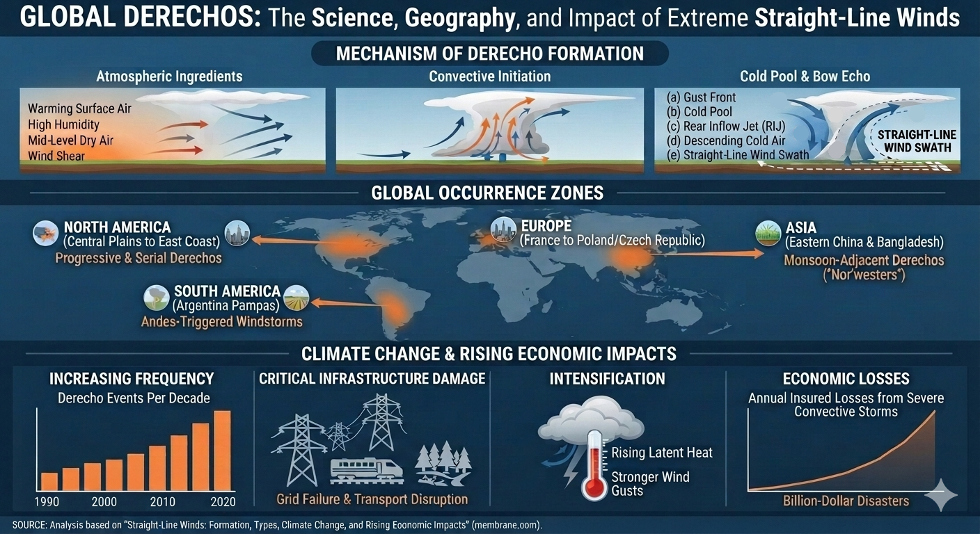
Although North America experiences some of the world’s most powerful and well-documented derechos, these storms are not unique to the United States. Derecho-like convective systems occur on nearly every continent and are increasingly being recognized in:
Central Europe
Eastern Asia
The subtropical plains of South America
As the global atmosphere continues to warm and store more moisture and energy, researchers are increasingly investigating whether the environmental conditions that support long-lived convective windstorms are becoming more common in regions that historically experienced them only rarely.
The expanding geographic footprint of derechos underscores a central lesson of climate science: severe weather hazards are not remaining stationary. As atmospheric energy increases, the boundaries of extreme events are shifting, exposing new populations, infrastructure, and economic systems to risks that were once considered geographically improbable.
Insurance Industry Responses
Global insured losses from severe convective storms are increasing at an estimated average annual rate of approximately 9%, substantially exceeding the growth rate of losses from other natural catastrophes.
In response, insurers are rapidly restructuring coverage across many regions of the United States.
Traditional policies that once contained flat-dollar wind deductibles are increasingly being replaced by percentage-based wind and hail deductibles ranging from 1% to 5% of a home’s insured value. These changes shift thousands of dollars of immediate disaster costs directly onto homeowners and businesses.
The insurance industry increasingly recognizes straight-line wind events not as isolated weather anomalies but as an emerging systemic risk requiring substantial adjustments in underwriting practices, pricing models, and catastrophe exposure management.
Conclusion: More Energy in the Atmosphere Means More Extreme Winds
Straight-line winds demonstrate a fundamental principle of climate physics: a warmer world is a more energetic world.
As greenhouse gases trap additional heat, the atmosphere stores more moisture and potential energy, creating increasingly favorable conditions for severe convective storms. The result is an environment capable of producing stronger downbursts, more frequent severe thunderstorms, and larger, longer-lived derecho systems.
Climate change does not cause any individual straight-line wind event in isolation. However, it is increasingly altering the environmental ingredients that govern these storms by increasing atmospheric moisture, elevating instability, and supporting more persistent convective systems.
The consequences extend well beyond meteorology. Straight-line winds are becoming a growing challenge for public safety, infrastructure resilience, electrical grid reliability, insurance markets, and building design standards. As the climate system continues to warm, understanding and preparing for these increasingly energetic wind events will become essential for protecting communities and reducing future economic losses.
What are the climate risks where you live?
Many people are surprised to learn that their greatest weather-related risk is often wind damage. Wind and hail damage are among the most common homeowners insurance claims in the United States, accounting for roughly 40% of all property damage claims.
Standard homeowners policies from major insurers generally cover wind damage under dwelling and personal property coverage. These claims can include repairs for roof and shingle damage, siding damage, structural failures, and damage caused by wind-driven debris such as fallen trees.
However, homeowners in high-risk areas—such as coastal regions and “Tornado Alley”—may face separate windstorm deductibles. Unlike a standard fixed deductible (for example, $1,000), these deductibles are often calculated as a percentage of the home’s insured value, typically ranging from 1% to 5%.
Complex social-ecological feedback loops arise when human systems and natural systems react to climate change in ways that amplify one another. Because Earth’s climate operates as a nonlinear system, these interactions do not unfold gradually — they can accelerate suddenly, compound unpredictably, and push the system toward irreversible shifts.
This nonlinear, cross-regional feedback behavior is something we have been modeling for decades — where climate physics couples directly with economic networks.
In the 1990s we underestimated one variable: human delay. We assumed mitigation would begin in earnest. It did not.
Now we observe potential doubling in the intensity or frequency of certain climate impacts on timescales of 2–10 years rather than centuries. The apparent acceleration has compressed from millennial-scale shifts to multi-decade nonlinear surges.
Denialism and Ecofascism
One factor we drastically underestimated was the influence of organized denialism and emerging ecofascist ideology.
Initially the investigation focused on a straightforward institutional question:
Were challenges to the EPA’s Endangerment Finding and coordinated regulatory rollbacks primarily driven by economic motives — specifically the fossil-fuel industry’s long-documented strategy of financing climate denial narratives?
Organizations such as the CO₂ Coalition and the Department of Energy’s Climate Working Group were key nodes of analysis. The economic motive was clear and well documented: protect fossil capital, delay regulation, and manufacture doubt.
But as correspondence, affiliations, and rhetoric were analyzed, a second pattern emerged.
This was not simply economic denialism. It was the normalization of ecofascist ideology.
Ecofascism reframes environmental collapse as beneficial — even desirable — if it reduces populations deemed inferior, excessive, or expendable. It merges environmental crisis with authoritarian hierarchy, racialized survival logic, and elite domination theory.
This is not speculation. It is visible in the language used by some elite circles revealed through the Epstein files.
Examples include statements attributed to Jeffrey Epstein such as:
“I liked the argument that more CO₂ is good for plants.”
“Maybe climate change is a good way of dealing with overpopulation — the Earth’s forest fire. Potentially a good thing for the species.”
Combined with statements reflecting explicit eugenic ideology:
“Executions of the elderly and infirm make sense.”
“African music has lots of beats and little development — no accident. It mirrors their learning process.”
This is not conventional policy disagreement. This is eliminationist logic.
Where traditional denial protects capital investment, ecofascism rationalizes unequal human survival.
“Climate change is increasing the amount of energy violent rain events contain, amplifying how much damage they can inflict.”
The physics of wind and rain are important to understand: their destructive force increases nonlinearly with velocity and is further amplified by density and mass. Even relatively small increases in wind speed or rainfall intensity can produce disproportionately larger impacts and damage.
This principle applies to all extreme energy events. At its core, climate change is an energy imbalance. As excess heat accumulates within the Earth system, more energy becomes available to drive storms, floods, droughts, heatwaves, and wildfires. As the energy intensifies, so do its manifestations.
The destructive power of both wind and water scales approximately with the square of velocity (v²), meaning relatively small increases in flow speed can lead to disproportionately large increases in force and damage. Density further amplifies these impacts. Because water is approximately 800 times denser than air, a 10 mph flow of water can exert roughly 800 times the force of a 10 mph wind at the same speed. As climate change increases flow velocities, the resulting forces and damages rise nonlinearly.
What does this mean? The physics of extreme events is nonlinear. Wind and water damage do not increase in a simple one-to-one relationship with climate change because destructive force scales with the square of velocity. As climate feedbacks become increasingly coupled, extreme events can become more intense, more frequent, and longer lasting. Climate change is not simply producing more storms or heavier rainfall; it is altering the physical conditions that determine how much energy these events contain and how much damage they can inflict.
Damages — The destructive power of moving water is evident in countless real-world examples. Floodwaters do not simply rise; they become a powerful moving force capable of transporting enormous amounts of mass and energy. Fast-moving water can:
Wash out bridges and roadways by scouring away foundations, eroding support structures, and undermining concrete, asphalt, and other infrastructure.
Carry away trees, vehicles, buildings, and debris, turning ordinary objects into battering rams that multiply destruction downstream.
Destroy homes and infrastructure as flood currents exert immense lateral pressure on walls, foundations, electrical systems, and utilities.
Trigger mudslides, debris flows, and landslides when saturated soils lose strength and entire hillsides collapse under the weight of water.
Cause catastrophic slope failures, where mountainsides, roads, and communities can be buried beneath rapidly moving earth, rock, and water.
Erode riverbanks and coastlines, permanently reshaping landscapes and removing natural protective barriers.
Damage dams, levees, and flood-control systems when water volumes and flow rates exceed engineering design limits.
Scour foundations and expose underground utilities, causing structural failures that can continue long after floodwaters recede.
Destroy agricultural land by stripping away fertile topsoil, depositing contaminated sediments, and altering drainage patterns.
Create deadly debris flows where water, soil, rocks, trees, and other materials combine into a dense, high-speed slurry capable of moving massive boulders and destroying entire neighborhoods.
The danger of extreme flooding is not only the amount of water involved, but the velocity and density of that water. Because water is hundreds of times denser than air, even relatively slow-moving floodwaters can generate forces capable of moving vehicles, uprooting trees, collapsing structures, and reshaping entire landscapes.
The aftermath of extreme flooding can create a second wave of destruction through cascading health impacts. When water treatment facilities fail, sewage systems overflow, and agricultural waste contaminates floodwaters, communities face increased risks from waterborne pathogens, bacterial infections, mold growth, toxic exposures, and disease outbreaks.
Floodwaters can also mobilize a complex mixture of chemical contaminants. Industrial facilities, warehouses, fuel storage tanks, landfills, mining sites, wastewater plants, and commercial properties may release petroleum products, pesticides, herbicides, fertilizers, solvents, heavy metals such as lead, mercury, and arsenic, and other hazardous chemicals into surrounding communities. Floodwaters can transport these contaminants over long distances, depositing them into homes, schools, agricultural fields, rivers, lakes, wetlands, and groundwater supplies.
As floodwaters recede, many contaminants remain behind in sediments, soils, and building materials. Some chemicals can become airborne as contaminated sediments dry, exposing people through inhalation as well as direct contact and ingestion. Certain toxins can persist in the environment for years, accumulate in food chains, contaminate crops and fisheries, and produce long-term ecological and human health consequences, including neurological disorders, respiratory illnesses, liver and kidney damage, developmental problems, reproductive effects, and increased cancer risks.
These cascading failures can overwhelm emergency services, disrupt drinking-water supplies, limit access to medical care, and create long-term public health challenges. The damage is therefore not limited to the immediate destruction caused by floodwaters; it can trigger a chain reaction affecting ecosystems, infrastructure, food systems, economies, and human health for months, years, or even decades afterward.
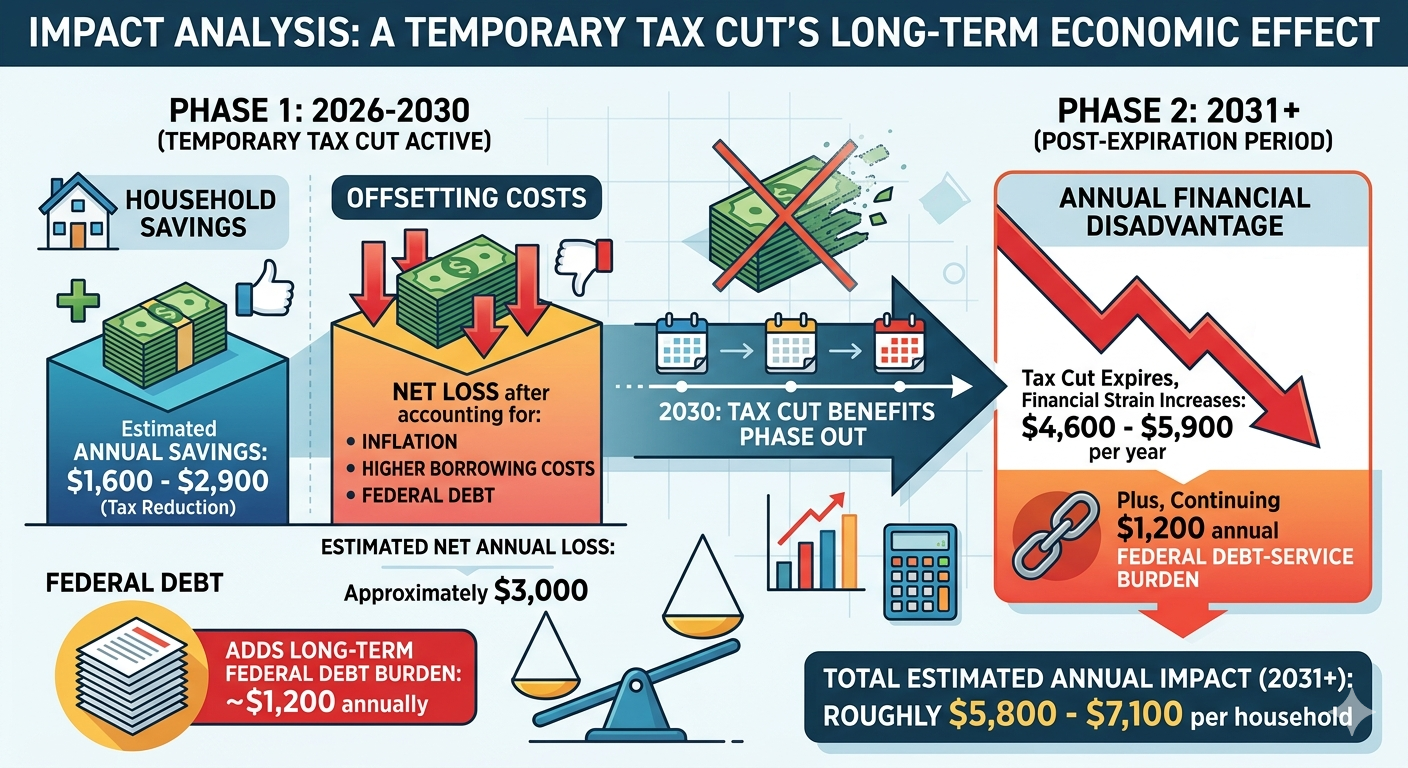
A tax cut that appeared to provide the average household with $1,600–$2,900 in annual savings was more than offset by the broader economic effects of inflation, higher borrowing costs, and increased federal debt. After accounting for these costs, the average household experienced an estimated net loss of approximately $3,000 per year, along with an additional long-term federal debt burden equivalent to roughly $1,200 annually.
However, the tax cut benefits are scheduled to phase out by 2030, meaning households will eventually lose the temporary savings while many of the costs associated with higher debt, interest payments, and elevated borrowing rates remain. Beginning in 2031, when the tax reduction expires, the average household’s annual financial disadvantage could increase to approximately $4,600–$5,900 per year, plus the continuing $1,200 annual federal debt-service burden. This would place the total estimated impact at roughly $5,800–$7,100 per household annually, while the accumulated federal debt continues to shift additional costs onto future taxpayers.
Tax Cuts vs. Inflation: The Hidden Battle Over Household Purchasing Power
Tax cuts are often promoted as a direct way to improve household finances, but for the average American family, inflation can have a much larger and more immediate impact on financial well-being. A tax cut may provide a noticeable boost to income, but a sustained period of elevated inflation can quietly reduce purchasing power by thousands of dollars each year.
For a typical middle-income household, a broad tax reduction might save several hundred to a few thousand dollars annually. However, inflation affects the entire household budget—including housing, groceries, utilities, transportation, healthcare, and services. A 4%–5% annual inflation rate can easily increase household expenses by $3,500–$5,000 per year, effectively overwhelming the benefit of many tax cuts.
The result is a simple economic reality: a dollar gained through tax cuts can be offset—or even erased—by dollars lost through higher prices.
The Mathematical Mismatch: Tax Savings vs. Inflation Costs
Tax Cuts Provide Limited Annual Gains
For most middle-class households, federal tax cuts typically produce moderate savings rather than dramatic changes in disposable income. Historical analyses of broad tax packages, including evaluations by organizations such as the Tax Policy Center, have shown that middle-income families often receive annual tax reductions in the range of roughly $1,600 to $2,900, depending on the structure of the legislation. The most recent tax cuts saved the average household $1,600 and $2,900.
While meaningful, these savings represent only a fraction of a household’s total annual expenses.
Inflation Acts Like a Hidden Tax
Inflation operates differently from taxes. Rather than reducing a paycheck directly, it increases the cost of nearly everything a household buys.
A family spending $80,000 annually on goods and services would experience approximately:
4% inflation: about $3,200 in additional annual costs
5% inflation: about $4,000 in additional annual costs
6% inflation: about $4,800 in additional annual costs
Unlike a tax cut, which may provide a one-time or annual benefit, inflation compounds year after year. Even if wages rise, households can still lose purchasing power if prices increase faster than incomes.
Distribution of Benefits vs. Distribution of Burdens
Tax Cuts Often Deliver Larger Dollar Benefits to Higher-Income Households
Income tax reductions generally scale with taxable income. Higher-income households typically pay more in taxes, so percentage-based tax cuts often produce larger dollar savings at the top.
Analyses from organizations such as the Congressional Budget Office have repeatedly shown that broad tax changes frequently provide the largest absolute benefits to higher-income groups, while middle- and lower-income households receive smaller dollar amounts.
Inflation Disproportionately Hurts Lower- and Middle-Income Families
Inflation is often described as a regressive economic force because it affects essential spending categories that consume a larger share of lower-income household budgets.
A wealthy household can often absorb higher prices by reducing discretionary spending or shifting purchases. A working-class family has fewer options when facing increases in:
Food prices
Rent or mortgage payments
Electricity and heating costs
Gasoline and transportation
Healthcare expenses
For families living close to their monthly budget limits, inflation functions like a pay cut.
The Inflation Feedback Loop
Tax cuts can stimulate economic activity by increasing disposable income. However, if tax reductions are not matched by spending reductions or productivity gains, they can increase demand in an economy already operating near capacity.
The mechanism is straightforward:
Tax cuts increase household disposable income.
Increased income boosts consumer demand.
If supply cannot expand quickly enough, businesses raise prices.
Higher prices reduce the purchasing power of the original tax cut.
In this scenario, households may receive additional money in their paycheck while simultaneously paying more at the grocery store, gas station, and utility bill.
The economic benefit becomes partially or completely offset by rising prices.
The Federal Debt Effect: How Tax Cuts Can Increase Long-Term Costs
Tax cuts also have a broader economic impact beyond the immediate benefit to taxpayers. When tax reductions are not accompanied by equivalent spending reductions or stronger economic growth, they increase the federal budget deficit and add to the national debt. The government must finance that additional debt by issuing more Treasury securities, increasing the supply of government borrowing.
As federal debt rises, the government competes with households and businesses for available capital. This increased demand for borrowed money can place upward pressure on interest rates, raising the cost of mortgages, auto loans, credit cards, business financing, and other forms of credit.
The effect is often indirect but significant. A household may receive a $2,000 annual tax reduction, but if higher federal borrowing contributes to even a modest increase in interest rates, that same family may pay thousands of dollars more over time through:
Higher mortgage rates when purchasing or refinancing a home
Increased interest on auto loans
Higher credit card balances
More expensive consumer financing
Higher costs passed through by businesses borrowing at elevated rates
For example, a 1% increase in mortgage rates on a $300,000 home loan can add roughly $200 per month to a typical 30-year mortgage payment—more than $2,000 annually. Across the economy, higher interest rates also increase the federal government’s own debt-service costs, requiring more taxpayer dollars to pay interest rather than fund public services or reduce future deficits.
This creates a potential feedback loop:
Tax cuts reduce federal revenue.
Larger deficits increase government borrowing.
Higher debt levels put upward pressure on interest rates.
Higher rates increase borrowing costs for households, businesses, and the government.
Additional interest expenses reduce the long-term economic benefit of the original tax cut.
The ultimate measure of a tax policy is therefore not only the size of the immediate tax reduction, but its effect on total household purchasing power after accounting for inflation, interest rates, and the long-term cost of increased federal debt.
The Role of Bracket Creep
Inflation also affects taxation through a process known as bracket creep.
As wages rise due to inflation, taxpayers can unintentionally move into higher tax brackets even though their real purchasing power has not increased. To address this, the Internal Revenue Service adjusts federal income tax brackets, standard deductions, and other thresholds annually for inflation.
These adjustments prevent inflation from automatically increasing a household’s tax burden. However, they do not compensate for the broader loss of purchasing power caused by rising prices.
Inflation indexing protects taxpayers from paying higher taxes simply because of inflation—it does not make groceries, housing, or energy affordable again.
Conclusion: The True Measure Is Total Economic Impact
Tax cuts can provide meaningful benefits to households, but their true economic value cannot be measured by the size of the immediate reduction in a tax bill alone. A complete evaluation must consider the broader effects on purchasing power, inflation, interest rates, and the long-term federal debt burden.
A tax cut may increase disposable income in the short term, but those gains can be diminished or even erased when inflation raises the cost of everyday necessities such as housing, food, energy, and transportation. Unlike a one-time tax reduction, inflation affects the entire household budget and compounds over time, reducing what each dollar can actually buy.
The impact also depends on how tax cuts are financed. When reductions in federal revenue are not matched by spending cuts or sufficient economic growth, they increase budget deficits and add to the national debt. Higher federal borrowing can place upward pressure on interest rates, increasing costs for mortgages, auto loans, credit cards, and business financing. Households may receive additional money through lower taxes while simultaneously paying more through higher borrowing costs and rising prices.
This creates a broader economic equation:
The benefit of a tax cut is not simply the dollars returned to taxpayers—it is the change in real purchasing power after accounting for inflation, interest rates, and future debt obligations.
For some households, especially higher-income taxpayers, tax reductions may provide substantial direct benefits. However, for many middle- and lower-income families, the effects of inflation and higher interest rates can outweigh those gains because they spend a larger share of their income on necessities and borrowing costs.
The ultimate question is therefore not:
“How much did taxpayers save in taxes?”
The more important question is:
“Did households become financially better off after accounting for the full economic consequences?”
A sustainable economic policy must balance tax relief with fiscal responsibility, price stability, and long-term economic growth. Without that balance, a tax cut can create the appearance of increased prosperity while shifting costs into higher prices, higher interest payments, and a larger debt burden for future generations.
ADDENDUM
The exact “net cost” depends on the household’s income, debt exposure, and whether the tax cuts are financed by borrowing. A reasonable estimate can be made by separating immediate annual effects from long-term debt effects.
Estimated Annual Impact on an Average Household
Item
Annual Impact
Tax cut benefit
+$1,600 to +$2,900
4% inflation increase in household expenses
−$3,200
Higher mortgage costs (if buying/refinancing)
−$2,000+
Higher auto loan, credit card, and consumer financing costs
−$500 to −$2,000+
Higher business borrowing costs passed through in prices
−$300 to −$1,000+
Additional federal debt interest burden
−$900 to −$1,500+ annually (estimated)
Short-Term Net Effect (First-Year Estimate)
Lower-cost scenario:
Tax savings: +$2,900
Inflation cost: −$3,200
Consumer borrowing/business costs: −$800
Debt interest effect: −$900
Net impact: approximately −$2,000 per household per year
Higher-cost scenario:
Tax savings: +$1,600
Inflation cost: −$3,200
Mortgage/borrowing costs: −$3,000
Debt interest effect: −$1,500
Net impact: approximately −$6,100 per household per year
Long-Term Federal Debt Effect
If tax cuts add $3–$5 trillion to federal debt:
There are roughly 130 million U.S. households.
The added debt equals approximately:
130 million households$3 trillion≈$23,000 per household130 million households$5 trillion≈$38,000 per household
That does not mean each household receives a bill, but it represents the additional federal liability ultimately supported by taxpayers.
If the government pays roughly 4% interest on that additional debt:
$3 trillion × 4% = $120 billion/year
$5 trillion × 4% = $200 billion/year
Spread across households:
$900–$1,500 per household annually in additional federal interest costs
Over decades, if the debt is refinanced and interest compounds, the total burden can become substantially larger.
Other Potential Costs Associated With Large Tax Cuts
1. Reduced fiscal flexibility
Higher debt can limit the government’s ability to respond to:
recessions
natural disasters
pandemics
military emergencies
infrastructure needs
Future taxpayers may face higher taxes or spending cuts to service the debt.
2. Higher interest rates
Large deficits can increase demand for borrowed funds, putting upward pressure on interest rates. This affects:
mortgages
business loans
student loans
auto loans
government borrowing costs
3. Crowding out private investment
When the government absorbs more available capital:
businesses may invest less
productivity growth can slow
wage growth may weaken over time
4. Inflation risk
If tax cuts increase demand without increasing supply, they can contribute to inflationary pressure, especially when the economy is already near capacity.
Estimated Net Household Effect
Time Frame
Estimated Impact
Immediate annual effect
−$2,000 to −$6,000 per household
Added federal debt liability
+$23,000 to +$38,000 per household
Annual debt-service burden
−$900 to −$1,500 per household/year
Bottom Line
A tax cut that appeared to provide an average household with $1,600–$2,900 in annual savings was far outweighed by the broader economic effects of inflation, higher borrowing costs, and increased federal debt. The average household had a net loss of $3,000 and an additional debt burden of $1,200/year. For many households, the combined impact may represent a net financial loss of several thousand dollars per year, while the long-term debt burden shifts additional costs onto future taxpayers.
A child’s financial future can be strengthened by using multiple savings vehicles, each designed for a different purpose. Rather than choosing only one account, families can combine them strategically to maximize government benefits, tax advantages, and long-term wealth creation.
Step 1: Capture the Free Government Contribution
For children born between 2025 and 2028, families should consider opening a Trump Account through Trump Accounts.gov as soon as possible to qualify for the initial $1,000 government contribution and any eligible corporate matching contributions.
The key advantage is that this initial deposit provides a foundation of invested capital that can compound for decades. When started early, even a relatively small contribution can grow substantially through the power of long-term investment returns.
Step 2: Use a 529 Plan for Education Savings
After securing available government contributions, families can direct additional college savings into a 529 education savings plan.
A 529 plan offers:
Tax-free growth on qualified education expenses
Tax-free withdrawals for eligible college, vocational, and educational costs
The ability for family members to contribute over time
For parents and grandparents specifically saving for education, a 529 plan remains one of the most efficient tools for building a dedicated education fund.
Step 3: Transition to a Custodial Roth IRA for Long-Term Wealth
Once a child has earned income from a legitimate job—such as babysitting, lawn care, summer employment, or other documented work—a Custodial Roth IRA can become a powerful wealth-building tool.
A Roth IRA allows:
Tax-free investment growth
Tax-free qualified withdrawals in retirement
The potential to use contributions (not earnings) later for certain purposes, such as a first-home purchase
Starting a Roth IRA during childhood gives decades of compounding potential and can help transform early earnings into a future home down payment or retirement asset.
The Three-Account Strategy: A Lifetime Financial Roadmap
The most powerful approach is not choosing between accounts—it is using each account for its intended purpose:
Trump Account → Capture free government and matching contributions
529 Plan → Build a tax-advantaged education fund
Custodial Roth IRA → Create lifelong tax-free wealth
By combining these tools, families can provide children with a financial foundation that supports education, home ownership, and long-term financial independence. The earlier the process begins, the greater the benefit of decades of compound growth.
I recently had a conversation with an author who described the painstaking process of publishing a book decades ago. The manuscript was written on an early Amstrad word processor. Each section had to be printed, physically cut with scissors, and glued onto format sheets provided by the publisher. Every chapter was constrained to a specific page count and layout. Photos and graphics required coded placeholders, separate lists of image requirements, rough sketches, and coordination with researchers and artists. It was an incredibly slow and labor-intensive process.
That story resonated deeply with me because I experienced similar challenges during the early days of the World Wide Web.
Around 1992, web engineering and publishing were equally demanding. Creating even a single graphic for a webpage could take weeks or months. The tools we take for granted today did not exist. There were no drag-and-drop interfaces, content management systems, or automated publishing platforms. Everything was handcrafted.
During that period, I created what I called the first web “button”—the Panic Button. The concept was simple: if someone didn’t know how to use the web, they could click on the graphic and receive help. In effect, it became the first World Wide Web help desk, designed to guide users through an entirely new digital environment.
The Panic Button represented something even more fundamental. It was the invention of the clickable image—an inline graphic with a hyperlink wrapped around it. Today, clickable images are so commonplace that they seem obvious, but at the time, the idea of turning an image itself into an interactive navigation element had not yet become part of the web experience. The button transformed a static picture into an action, helping establish the principle that graphics could serve not merely as illustrations but as gateways to information and services.
The original Membrane website can still be viewed at:
Our work extended beyond web development. We were also among the early record companies on the web, experimenting with concepts that would eventually become commonplace, including music subscriptions, pay-per-download services, and streaming media. I found music production particularly rewarding, and advances in technology allowed me to dramatically increase my creative output.
In the early years, I produced approximately fifty songs per year. As digital tools improved, that number increased to around one thousand songs annually between 1992 and 2023. Today, with AI-assisted composition, production software, and modern mastering technologies, I can publish approximately 7,300 songs per year at substantially higher levels of production and mastering quality. Measured purely by output, that represents a 146-fold increase in productivity.
Scientific publishing has undergone a similar transformation. Much of climate science involves mathematical analysis, data processing, modeling, and the communication of complex ideas. A scientific paper that once might have required a year of calculations, drafting, revisions, graphics production, and formatting can now often be completed in a matter of days.
The significance of these technological changes extends beyond simple speed. Technology has compressed production timelines while simultaneously improving quality and dramatically expanding the capabilities of individuals. Tasks that once required teams of specialists and months of effort can increasingly be accomplished by a single person equipped with modern digital tools and artificial intelligence.
Having lived through both eras—the age of scissors and glue sticks and the age of AI-assisted creation—the contrast is remarkable. We have witnessed one of the greatest productivity revolutions in human history, one that has fundamentally transformed publishing, music, science, and the very process of turning ideas into reality.
The unexpectedly rapid release of more than $100 billion in tariff refunds is likely amplifying an already sharp increase in U.S. imports, contributing to a much wider trade deficit reported today by the Bureau of Economic Analysis.
According to the U.S. Bureau of Economic Analysis (BEA), the international trade deficit jumped 42.2% to $77.6 billion in May, up from a revised $54.6 billion in April. Imports climbed 3.3% to $395.3 billion, while exports fell 3.2% to $317.7 billion.
While businesses also accelerated purchases ahead of potential new tariffs and supply chain disruptions, the rapid release of tariff refunds appears to have become a major source of liquidity that enabled importers to dramatically increase orders from overseas.
Tariff Refunds Are Moving Much Faster Than Expected
The current refund program stems from the February 2026 U.S. Supreme Court ruling that invalidated many emergency tariffs imposed under the International Emergency Economic Powers Act (IEEPA). Since then, U.S. Customs and Border Protection (CBP) has been processing one of the largest customs refund programs in U.S. history.
The pace of payments has exceeded many expectations:
Approximately $166 billion in refund claims have been filed.
More than $104.3 billion has already been accepted.
Roughly $71 billion has been finalized and paid.
On June 29, CBP launched Phase 2 of its automated CAPE refund portal to process an additional 2.8 million older and more complex import entries.
The unexpectedly rapid return of more than $100 billion to importers has significantly improved corporate cash flow, allowing companies to replenish inventories and increase imports almost immediately.
Refund Liquidity Is Expanding the Trade Deficit
The refund process has created a powerful economic chain reaction:
More than $104 billion in accepted refund claims → Increased importer liquidity → Accelerated foreign purchasing → Larger U.S. trade deficit
Instead of remaining tied up in government accounts, tariff revenue is now flowing back into corporate balance sheets, enabling businesses to front-load imports while attempting to stay ahead of replacement tariff policies.
Tariff Revenue Has Effectively Disappeared
The refund program is also dramatically reducing federal customs revenue.
In May 2026, the U.S. Treasury paid out $21.97 billion in tariff refunds while collecting $21.93 billion in gross customs duties. The result was a net customs outflow of approximately $42 million, effectively eliminating tariff revenue for the month.
Growing Pressure on the Federal Budget
The reversal from collecting tariffs to issuing massive refunds is widening the federal fiscal deficit.
Because tariffs had become a significant source of government revenue, refunding those collections represents both a loss of expected receipts and a substantial increase in federal expenditures.
Moody’s Analytics estimates the immediate fiscal impact could exceed $133 billion.
The Congressional Budget Office (CBO) projects that related policy changes could increase federal deficits by roughly $2 trillion over the next decade.
Consumers See Little Benefit
Although corporations are receiving billions in refund payments, consumers are unlikely to see corresponding price reductions.
Several major retailers—including Nike, Amazon, and Costco—are facing class-action lawsuits alleging they retained tariff-related price increases while also receiving refund payments, allowing them to benefit from both higher prices and government reimbursements.
New Tariffs Could Offset the Windfall
Following the Supreme Court decision, the U.S. Trade Representative introduced new tariffs under alternative statutory authorities, including Section 122 and Section 301.
Many importers warn that these replacement tariffs could quickly erode the financial gains created by the current refund program. In the meantime, however, the rapid pace of tariff refunds is injecting substantial liquidity into import markets, contributing to a wider trade deficit and placing additional pressure on the federal budget.
Global warming is often communicated through changes in average surface air temperature. While useful, this framing understates the fundamental driver of climate change: the accumulation and redistribution of excess thermal energy throughout the Earth system. Because more than 90% of anthropogenic excess heat is stored in the oceans, surface temperature alone provides only a partial representation of the climate system’s changing energy balance. We argue that conceptual illustrations of climate change should therefore be interpreted as probability distributions of total climate-system energy rather than simple temperature distributions. As Earth’s energy imbalance increases, the statistical distribution of climate outcomes evolves beyond a simple rightward shift. The distribution becomes increasingly skewed, with a broader and heavier upper tail corresponding to more frequent, more intense, and longer-duration extreme events. Simultaneously, individual hazards increasingly interact through nonlinear feedback coupling, producing compound and cascading extremes. These changes reflect the redistribution of excess thermal energy through atmospheric and oceanic processes rather than isolated changes in weather. Understanding climate change as an evolving probability distribution governed by Earth’s energy imbalance provides a more comprehensive framework for interpreting modern climate extremes.
1. Introduction
Climate change is frequently illustrated using a bell-shaped probability distribution in which warming shifts the distribution toward higher temperatures, increasing the likelihood of extreme heat events. Although this visualization effectively introduces the concept of changing probabilities, it risks oversimplifying the underlying physics.
The Earth’s climate is fundamentally governed by its energy balance. Anthropogenic greenhouse gases reduce outgoing longwave radiation, producing a persistent planetary energy imbalance. Most of this excess energy is not retained in the atmosphere but absorbed by the oceans, which currently store more than 90% of the additional heat accumulating in the climate system (von Schuckmann et al., 2023; IPCC, 2021).
Consequently, a conceptual continuum extending from lower to higher thermal energy more accurately represents climate-system evolution than one depicting air temperature alone. The atmosphere, oceans, cryosphere, biosphere, and land surface collectively exchange this stored energy through complex interactions that manifest as increasingly energetic weather events.
2. Earth’s Energy Imbalance as the Primary Climate Variable
Surface air temperature is an important diagnostic variable but represents only a small fraction of the total energy accumulating within the Earth system.
Recent observations indicate that the planetary energy imbalance has increased substantially over the satellite era (Loeb et al., 2021). Excess energy is partitioned approximately as follows:
Reservoir
Approximate Fraction of Excess Heat
Oceans
>90%
Land
~5%
Ice Melt
~3%
Atmosphere
~1%
Because the oceans dominate planetary heat storage, climate evolution is fundamentally an energetic process rather than merely an atmospheric warming process.
The horizontal axis in conceptual probability diagrams should therefore be interpreted as representing increasing Earth-system thermal energy, encompassing ocean heat content, atmospheric moisture, latent heat, and the energy available to drive weather systems.
3. Evolution of the Probability Distribution
Traditional illustrations depict warming primarily as a rightward shift of a normal distribution.
However, observations increasingly indicate that the distribution itself is evolving.
Rather than simply translating toward warmer conditions, the upper tail is becoming:
longer,
broader,
heavier,
increasingly asymmetric.
Statistically, this reflects increasing positive skewness and changes in higher-order moments of the climate distribution.
The consequence is that events formerly located far within the statistical tail now occur substantially more often than predicted by historical climatology.
This evolution is consistent with attribution studies demonstrating rapidly increasing probabilities for extreme heat, heavy precipitation, marine heatwaves, and compound climate events (IPCC, 2021).
4. From Rare Extremes to Persistent Extremes
A critical consequence of distributional change is that climate extremes are no longer simply more intense.
They also persist longer.
Persistent blocking highs and heat domes illustrate this transition.
Recent heat events across North America and Europe have demonstrated that elevated temperatures sustained over many consecutive days produce disproportionately greater impacts than isolated hot days.
Long-duration heat increases:
cumulative physiological stress,
nighttime heat exposure,
agricultural losses,
wildfire potential,
electrical demand,
ecosystem mortality.
The probability distribution therefore evolves not only along the intensity axis but also along the temporal dimension.
Duration has become an equally important component of climate risk.
5. Probability Distributions Represent Climate Outcomes, Not Individual Weather Variables
The conceptual bell curve should not be interpreted as describing only hot versus cold weather.
Rather, it represents a simplified probability density distribution of climate outcomes.
The horizontal axis encompasses the full spectrum of possible climate states, while the vertical axis represents their relative probability of occurrence.
Individual manifestations include:
heat waves,
atmospheric rivers,
tropical cyclones,
drought,
severe thunderstorms,
flooding,
wildfire weather,
marine heatwaves,
compound events.
Each reflects a different pathway through which excess thermal energy is redistributed throughout the coupled Earth system.
6. Feedback Coupling and Increasing System Connectivity
Perhaps the most important characteristic of the modern climate system is not simply increasing extremes but increasing interdependence among extremes.
Historically, many weather hazards could be treated as relatively independent processes.
As planetary energy accumulates, however, nonlinear interactions become increasingly common.
Warmer oceans provide additional latent heat to tropical cyclones.
Persistent blocking strengthens heat domes.
Elevated instability increases severe convection and lightning.
Drought increases wildfire probability.
Wildfires increase atmospheric aerosols and carbon emissions.
Ice loss reduces albedo, increasing additional heat absorption.
These interactions represent examples of feedback coupling, whereby one climate process amplifies another through interconnected physical mechanisms.
Rather than isolated hazards, modern climate extremes increasingly function as components of a dynamically coupled energetic system.
7. Earth’s Energy Redistribution
The planetary energy imbalance itself cannot be directly perceived.
Its consequences, however, are observable through increasingly energetic transfers of heat within the climate system.
These transfers manifest as:
stronger atmospheric rivers,
larger heat domes,
heavier precipitation,
more intense tropical cyclones,
stronger thunderstorms,
increased lightning,
more persistent drought,
expanded wildfire activity.
Each represents a different mechanism by which excess thermal energy is redistributed throughout the atmosphere-ocean system.
Viewed collectively, these events provide tangible evidence of an increasingly energetic climate.
8. Implications for Climate Communication
Public discussion frequently emphasizes average warming.
While scientifically accurate, averages obscure the statistical transformation occurring within climate variability.
The central message is therefore not simply that the planet is becoming warmer.
Rather, the probability distribution governing climate outcomes is itself evolving.
Extreme events once considered exceptionally rare now occur with increasing frequency, persist for longer durations, and produce substantially greater societal, ecological, and economic impacts.
Communicating climate change through the lens of Earth’s changing probability distribution provides a more complete understanding of modern climate dynamics than average temperature alone.
9. Conclusion
The defining characteristic of contemporary climate change is not simply rising global mean temperature, but the accumulation and redistribution of excess thermal energy throughout the coupled Earth system. Because the oceans absorb the overwhelming majority of this excess heat, Earth’s energy imbalance provides a more physically meaningful framework for understanding climate evolution than atmospheric temperature alone.
As this energy imbalance grows, the probability distribution of climate outcomes undergoes a fundamental transformation. The distribution does not merely shift toward warmer conditions; it becomes increasingly asymmetric, with a broader and heavier upper tail reflecting more frequent, more intense, and more persistent extreme events. At the same time, individual hazards are becoming progressively interconnected through nonlinear feedback coupling, allowing one extreme to amplify another across atmospheric, oceanic, terrestrial, and cryospheric systems.
Heat domes, atmospheric rivers, severe thunderstorms, tropical cyclones, droughts, floods, and wildfires should therefore be viewed not as isolated phenomena, but as diverse expressions of the same underlying energetic imbalance. Each represents a pathway through which excess thermal energy is redistributed across the Earth system. Interpreting climate change through this probabilistic and energetic framework provides a more comprehensive understanding of why extreme events are accelerating, why compound hazards are becoming increasingly common, and why climate impacts are intensifying faster than changes in global mean temperature alone would suggest.
Footnotes
Earth’s Energy Imbalance (EEI) is defined as the difference between incoming absorbed solar radiation and outgoing longwave radiation at the top of the atmosphere. A positive imbalance indicates continued accumulation of heat within the climate system.
Ocean heat content is widely regarded as the most robust measure of long-term planetary warming because it integrates the vast majority of excess thermal energy stored in the climate system.
In statistical terms, a “heavier right tail” denotes an increased probability of extreme positive departures relative to a normal distribution. In climate science, this reflects a greater likelihood of unusually intense events than would be expected under historical climatic conditions.
Feedback coupling refers to the interaction of two or more climate processes in which one process modifies another, producing amplification or attenuation. Positive feedback coupling can generate compound and cascading extremes that exceed the impacts of individual hazards.
Intergovernmental Panel on Climate Change (IPCC). (2021). Climate Change 2021: The Physical Science Basis. Cambridge University Press.
Loeb, N. G., et al. (2021). Satellite and ocean data reveal marked increase in Earth’s heating rate. Geophysical Research Letters, 48(8), e2021GL093047.
Rohde, R. A., & Hausfather, Z. (2020). The Berkeley Earth land/ocean temperature record. Earth System Science Data, 12, 3469–3479.
Trenberth, K. E., Fasullo, J. T., & Balmaseda, M. A. (2014). Earth’s energy imbalance. Journal of Climate, 27(9), 3129–3144.
von Schuckmann, K., et al. (2023). Heat stored in the Earth system 1960–2020: Where does the energy go? Earth System Science Data, 15, 1675–1709.
World Meteorological Organization (2024). State of the Global Climate 2024. Geneva: WMO.