bookmark_borderThe Presidency for Profit: Trump’s Conflicts of Interest, Financial Entanglements, and the Erosion of Public Accountability

Introduction: When Public Office Becomes a Private Business

Investigations, congressional probes, court proceedings, investigative journalism, and government watchdog reports have documented a disturbing pattern of alleged conflicts of interest, self-enrichment, and ethical violations involving Donald Trump. The controversies span both his first and second presidential terms, repeatedly centering on the intersection of presidential power, private business ventures, foreign financial relationships, and personal gain.

Organizations such as Citizens for Responsibility and Ethics in Washington (CREW), congressional oversight committees, and independent journalists have examined how Trump’s refusal to divest from his business empire created opportunities for political patronage, foreign influence, and financial conflicts. During his second term, cryptocurrency ventures and international business expansion have introduced additional avenues for private profit while his administration exercises regulatory, diplomatic, and economic power.

The pattern raises a fundamental question: Has Trump transformed the presidency into a mechanism for enriching himself, his family, political allies, and business associates while weakening the institutions designed to hold government officials accountable?

The controversies below illustrate the scope of these concerns.

1. Private Business Exploitation and Presidential Patronage

Conflicts of interest at Trump properties

During Trump’s first term, CREW tracked thousands of conflicts of interest stemming from his refusal to divest from his business empire. Its investigations documented visits to Trump properties by executive-branch officials, members of Congress, and foreign government representatives, including 145 foreign officials from 75 countries.

CREW’s reporting identified 3,403 distinct conflicts of interest in its earlier accounting. The broader record of presidential visits, political events, foreign-government spending, and official promotion of Trump properties illustrates how frequently public office intersected with private commercial interests.

The arrangement created an obvious incentive problem: officials and organizations seeking access to the president could direct business toward properties from which he benefited financially. Foreign governments and domestic political interests could spend money at Trump-owned venues while simultaneously seeking favorable treatment from his administration.

Political events and private revenue

Political groups and special interests reportedly held 319 events at Trump-branded properties, directing more than $23.2 million in revenue into his private businesses.

The underlying concern is straightforward. A president should not have a financial incentive to favor organizations, donors, lobbyists, or foreign representatives because they patronize his businesses. Yet Trump’s ownership structure allowed political activity and commercial revenue to converge.

During his second term, the problem expanded beyond traditional hotels and golf courses. His cryptocurrency ventures, international licensing arrangements, and other Trump-branded enterprises created additional opportunities for individuals and organizations to establish financial relationships with businesses associated with the president.

CREW’s second-term tracking has documented continued visits by foreign officials, political events at Trump properties, and official promotion of his businesses. These are not merely hypothetical conflicts. They are recurring features of a presidency in which private commercial interests remain intertwined with public responsibilities.

Taxpayer-funded promotion of Trump properties

Trump spent a substantial portion of his first presidency visiting his own golf courses and resorts. Those trips required the Secret Service and other government personnel to incur expenses at properties he owned. Watchdog estimates placed Secret Service and related spending at Trump properties at more than $1.1 million.

Taxpayers must pay to protect the president wherever he travels. But when presidential travel generates revenue for the president’s own businesses, public expenditures can become private commercial benefits.

The arrangement creates a conflict regardless of whether individual security expenditures were justified. The president’s private businesses can receive revenue because the government must provide security, while taxpayers bear the costs.

This is precisely why divestment and independent financial safeguards matter. Without them, the president’s personal financial interests remain embedded in the ordinary operations of government.

2. Cryptocurrency: A New Avenue for Presidential Self-Enrichment

Trump’s cryptocurrency ventures have dramatically expanded the potential financial conflicts associated with his presidency. World Liberty Financial, the $TRUMP memecoin, and related family-backed enterprises have created opportunities for substantial revenue from investors whose identities, motivations, and relationships with the administration deserve scrutiny.

Congressional Democrats and investigative reports have alleged that foreign nationals, corporate entities, and politically connected investors directed money into Trump-associated cryptocurrency ventures while the administration pursued regulatory changes favorable to the digital-asset industry.

Money flowing toward Trump while policy changes benefit the industry

The House Judiciary Committee Democrats have alleged that foreign financial backers of Trump-family cryptocurrency ventures received favorable regulatory treatment, policy changes, and the termination of federal investigations involving major industry participants.

The companies and cases discussed in this controversy include Coinbase, Kraken, and Ripple. The allegations concern whether enforcement decisions and regulatory rollbacks were made independently or whether the administration’s policies were influenced by the financial interests of Trump and his associates.

The potential conflict is especially serious because Trump is not merely a president overseeing an industry in which he has an incidental investment. His family-linked ventures have generated substantial revenue from cryptocurrency products while his administration has promoted the industry and changed its regulatory environment.

In such circumstances, investors may have financial reasons to support Trump-associated ventures beyond the expected commercial return. A financial relationship can also provide an avenue for cultivating access to the president.

The quid pro quo question

The central allegation is that financial contributions or investments flowed toward Trump-associated enterprises while the administration delivered regulatory benefits to the industry and its participants.

If established, such an arrangement would represent a profound corruption of the relationship between public policy and private enterprise. It would mean that a president’s financial interests and the interests of his investors were potentially advancing together through government action.

The administration and its supporters may characterize these policies as legitimate efforts to promote innovation and reduce regulatory burdens. But that explanation does not eliminate the conflict created when the president and his family stand to profit from the same industry affected by those decisions.

The appropriate question is not whether cryptocurrency regulation should be more permissive or more restrictive. It is whether the president’s financial interests have compromised independent policymaking, impartial enforcement, or national security.

3. Foreign Gifts, International Deals, and Potential Emoluments Violations

Foreign governments and valuable gifts

Trump’s receipt of valuable benefits associated with foreign governments and business interests has raised serious questions about the Constitution’s Foreign Emoluments Clause and the safeguards intended to prevent foreign influence over American officials.

Among the arrangements that have attracted scrutiny are a Boeing 747 valued at approximately $400 million offered by Qatar for presidential use, a gold bar reportedly valued at $130,000 associated with Swiss business interests, and a jeweled ring associated with a Belgian diamond group.

Critics have also questioned the timing of certain gifts and commercial arrangements relative to changes in U.S. tariff policy affecting the countries involved.

The concern is not simply that a president receives something valuable. It is that foreign governments and politically connected business interests may provide benefits to a president whose decisions affect their economic and strategic interests.

A gift does not automatically prove a corrupt bargain. But valuable benefits, opaque arrangements, and favorable government decisions occurring within the same financial and political relationships warrant rigorous investigation. The relevant questions include who provided the benefits, who ultimately received them, what disclosures were made, and whether official decisions were influenced.

Jared Kushner: Diplomacy and foreign sovereign wealth

CREW has challenged Jared Kushner’s role as a volunteer international envoy without Senate confirmation, arguing that his diplomatic responsibilities raise questions about applicable ethics and financial-disclosure requirements.

The controversy is particularly significant because Kushner’s private-equity firm, Affinity Partners, has attracted billions of dollars in investment commitments from foreign sovereign wealth funds, including Saudi Arabia’s Public Investment Fund.

The overlap between private investment and international diplomacy creates a serious conflict-of-interest concern. Kushner and other Trump associates have participated in sensitive Middle East diplomacy while maintaining financial relationships with foreign investors whose governments have substantial interests in U.S. foreign policy.

When private investment managers participate in negotiations involving governments that finance their businesses, the public has legitimate reasons to question whether private financial incentives could affect public decisions.

The issue is not resolved by describing an envoy as a volunteer or a private citizen. The substance of the responsibilities, the relationships involved, and the applicable legal requirements must determine what safeguards are necessary.

Donald Trump Jr., Eric Trump, and foreign mineral deals

Investigative reporting has also examined Trump-family business interests involving foreign mining and critical-mineral opportunities, including reported advisory roles and equity stakes associated with international corporate ventures.

These relationships become particularly consequential when family members stand to benefit from commercial opportunities while the presidential administration negotiates trade agreements, mineral-access arrangements, or other multibillion-dollar deals with foreign governments.

The resulting conflict is difficult to dismiss. Government policy can influence the value of private investments, while the people benefiting from those investments have close personal and business relationships with the president.

The question is whether the administration’s decisions are being made solely in the national interest or whether family business opportunities have become an additional consideration.

4. Presidential Clemency for Sale: The Pay-to-Play Problem

The presidential pardon power is broad, but its exercise can still become a vehicle for political favoritism and influence-peddling.

Investigative reporting has described an informal clemency channel through which wealthy individuals and politically connected offenders have sought presidential pardons outside conventional Department of Justice review procedures. Reports have described lobbyists and intermediaries charging fees of $1 million or more, with some clients reportedly offering substantially larger success fees.

The controversy is not that attorneys charge for legal services or that presidents grant controversial pardons. It is the possibility that individuals with sufficient wealth and privileged access can bypass ordinary procedures and obtain clemency through personal or political connections.

The pardon of Binance founder Changpeng Zhao intensified these concerns because of the company’s connections to the broader Trump-family cryptocurrency business environment. The sequence of business relationships, lobbying activity, and clemency raised questions about whether private financial interests and presidential discretion had become dangerously intertwined.

A system in which wealthy offenders can purchase access to the president through intermediaries threatens the principle that justice should not depend on personal wealth or political connections.

Where payments, lobbying relationships, and pardons intersect, the public deserves a transparent accounting of who paid whom, what was promised, who participated in the process, and why the pardon was granted.

5. Suing the Government, Rewarding Allies, and Dismantling Oversight

Seeking taxpayer-funded settlements from agencies Trump controls

Trump has pursued legal claims against federal agencies, including the FBI and Department of Justice, over investigations involving him. Reports have discussed potential claims reaching approximately $230 million.

The arrangement creates an extraordinary conflict: Trump is simultaneously the plaintiff seeking compensation and the president overseeing the executive branch responsible for defending the government against his claims.

That conflict becomes more troubling when the agencies involved are headed by officials appointed by the person seeking the money. Even if a legal claim has merit, the process must be independent enough to prevent presidential authority from influencing the government’s defense or settlement decisions.

The controversy surrounding a proposed $1.8 billion federal fund associated with legal claims involving Trump and his political supporters raised similar concerns. The proposal drew substantial criticism over its structure, potential beneficiaries, and implications for public accountability before congressional backlash forced its abandonment.

The danger is clear: the federal government must not become a mechanism through which a president can use executive authority to direct public resources toward himself or his political allies.

Removing the people responsible for exposing misconduct

After returning to office, Trump rescinded Biden-era ethics commitments that restricted political appointees from participating in matters involving their former lobbying clients. He also terminated numerous federal inspectors general and removed the head of the Office of Government Ethics.

Inspectors general investigate waste, fraud, abuse, and misconduct within federal agencies. Government ethics officials help ensure that public employees comply with rules designed to prevent conflicts of interest and misuse of public office.

Removing these officials weakens the institutional safeguards intended to expose corruption and hold government personnel accountable. The consequences extend beyond any individual investigation: fewer independent watchdogs mean fewer opportunities to identify conflicts, preserve evidence, and correct abuses of authority.

A president who benefits financially from private business relationships has an especially strong obligation to preserve independent oversight. Weakening that oversight while expanding private financial interests creates a dangerous concentration of power.

6. Trump’s Bankruptcies, the Road to Russia, and Foreign Financial Leverage

The relationship between Trump’s business history and Russia deserves particular attention when evaluating his foreign-policy decisions and the recurring controversy surrounding his treatment of Vladimir Putin.

Trump’s long record of corporate bankruptcies and restructurings matters because it shaped his business relationships with lenders, investors, and financial partners. His casino and real-estate ventures generated substantial losses for creditors and investors, while repeated financial difficulties complicated his access to conventional financing.

After years of troubled business ventures, Trump faced a narrower and more complicated financing environment. Traditional lenders were not always willing to provide the terms he wanted, creating incentives to seek alternative investors, private lenders, international partners, and intermediaries.

This is where the Russia connection becomes relevant.

Trump SoHo and Russian-linked money

The Trump SoHo development in New York became a focus of scrutiny because of its investors, business partners, and financing relationships. The project was associated with Felix Sater, a businessman with a criminal history who played a role in Trump-related real-estate ventures.

Investigative reporting and public allegations raised questions about Russian-linked money, Eastern European financial connections, and the possibility that luxury real-estate transactions could provide channels for moving funds of questionable origin.

The broader concern is that opaque financial arrangements can conceal the identities of investors, the sources of capital, and the interests of those providing financing. Shell companies and intermediaries can make it difficult to establish who ultimately benefits from a transaction.

The allegations surrounding Trump-related projects warrant scrutiny, but they must be distinguished from a proven finding that a specific transaction constituted money laundering. The relevant financial records, ownership structures, and evidence of criminal intent determine what can be established in each case.

Financial dependence creates potential leverage

The underlying economic principle is straightforward: when conventional financing becomes difficult to obtain, a businessperson may become more dependent on investors willing to accept greater risks or pursue less conventional arrangements.

That dependence can create vulnerabilities, particularly when the sources of financing are opaque or connected to foreign political and business networks.

It does not automatically prove that an investor controls the borrower or that a foreign government can dictate the borrower’s political decisions. But it creates a legitimate reason to investigate financial relationships, potential obligations, undisclosed liabilities, and possible sources of leverage.

For a president, the stakes are substantially higher than for an ordinary businessperson. Presidential decisions affect sanctions, international trade, military assistance, diplomatic recognition, and national security. Financial relationships that might be a private business concern in another context can become matters of national interest when the person involved occupies the Oval Office.

From financial vulnerability to questions about Putin

Critics have long questioned Trump’s unusually deferential treatment of Putin and his repeated willingness to challenge assessments or positions advanced by American intelligence agencies and traditional U.S. allies.

That criticism has acquired a particularly sharp expression in the phrase “Putin’s little bitch”—a crude political characterization of what critics perceive as Trump’s deference to the Russian president.

The phrase is deliberately blunt, but the underlying question is serious: Could financial vulnerabilities, personal interests, or other relationships help explain Trump’s approach to Putin and Russia?

That question cannot be answered by rhetoric alone. It requires examining documented financial records, business relationships, public statements, diplomatic decisions, and the treatment of Russian interests by the administration.

Nevertheless, it would be equally mistaken to dismiss the question simply because financial leverage has not been established in every instance. The possibility of undisclosed obligations or foreign influence is precisely why transparency and independent investigation are essential.

The implications for peace negotiations and Ukraine

The same questions arise whenever Trump negotiates with Russia over Ukraine or presents a diplomatic initiative as a peace agreement.

A proposed agreement should be evaluated by its terms, the concessions demanded from each side, the security guarantees provided, and the consequences for American interests and European stability.

But when credible questions exist about a president’s foreign financial relationships or potential vulnerabilities, those questions become relevant to the evaluation of his diplomacy. They cannot simply be dismissed as partisan attacks.

The concern is not that every concession to Russia must be corrupt. Diplomacy necessarily involves compromise. The concern is whether decisions are being made for defensible national-security reasons or whether undisclosed personal, financial, or political considerations are influencing the outcome.

A president’s duty is to the United States, not to foreign investors, private business partners, family enterprises, or personal relationships with foreign leaders.

Conclusion: The Convergence of Money, Power, and Political Accountability

Taken together, the controversies surrounding Trump’s business empire, cryptocurrency ventures, foreign gifts, international investments, presidential pardons, legal claims, and treatment of oversight institutions reveal a recurring pattern: the potential convergence of private financial gain and public power.

The individual controversies differ in their evidence and legal status. Some involve documented transactions or official actions; others involve allegations, unresolved legal questions, or interpretations of motive. But the cumulative effect is a fundamental challenge to public confidence in the presidency.

When a president retains substantial private business interests, foreign governments and wealthy investors have opportunities to establish financial relationships with those interests. When regulatory decisions, diplomatic negotiations, pardons, and government settlements occur within the same political environment, the need for independent scrutiny becomes even more urgent.

When inspectors general and ethics officials are removed, the institutions responsible for investigating misconduct become weaker. When public resources and executive authority can potentially benefit the president, his family, or his political allies, the distinction between governing and private enrichment becomes increasingly difficult to maintain.

The danger is not limited to one individual or one administration. It is the possibility of an American political system in which wealth purchases access, access creates influence, influence produces favorable decisions, and weakened oversight prevents the public from determining how those decisions were made.

That is the central concern behind the allegations of presidential profiteering and foreign financial influence. It is also why transparency, independent oversight, and the rule of law are essential to democratic government.

The presidency is a public trust, not a private investment vehicle. The American government must serve the public interest—not become a mechanism for enriching the people who control it.
bookmark_borderHow Long COVID May Affect Memory Through the Gut

by Daniel Brouse

A University of Pennsylvania study suggests that persistent COVID-related changes in the gut may contribute to memory problems and brain fog in some people with long COVID by reducing serotonin, a chemical messenger involved in communication between the gut and brain.

The proposed chain of events

  1. The virus persists: Researchers found traces of SARS-CoV-2 in the stool of some long COVID patients months after infection, suggesting that the virus may remain in the gut.
  2. Inflammation continues: Persistent viral material may keep the immune system activated, causing ongoing inflammation.
  3. Serotonin production falls: Inflammation may interfere with the gut’s ability to absorb tryptophan, an essential building block for serotonin.
  4. Gut–brain communication is disrupted: Lower serotonin may affect signaling through the vagus nerve, which carries information between the gut and brain.
  5. Memory may suffer: Experiments in mice linked this pathway to memory problems. Boosting serotonin using tryptophan-related compounds or SSRI antidepressants improved memory in the animals.

Why the findings matter

The research identifies a possible biological link between persistent gut infection, inflammation, reduced serotonin, and neurological symptoms. If confirmed in humans, serotonin levels might eventually help researchers identify a subset of long COVID patients who could benefit from targeted treatment.

Important limitations

  • The pathway appears to affect only a subset of people with long COVID.
  • Although researchers found associations in human patients, key cause-and-effect relationships were demonstrated in mice.
  • Long COVID likely has multiple biological causes, so this mechanism cannot explain every case of brain fog or memory impairment.
  • Clinical trials are needed to determine whether SSRIs or supplements are safe and effective for treating these symptoms.

Bottom line: The study offers a plausible explanation for how long COVID may affect memory through the gut–brain connection. It is an important research lead, not yet proof that low serotonin causes brain fog in people or that raising serotonin will treat it. SSRIs and supplements should not be started for long COVID without medical guidance.

Original Research

COVID (and other conditions) destroys good gut bacteria resulting in a compromised immune system. Gut bacteria play several key roles in your health that include communicating with your immune system and producing vitamins. Without good gut bacteria it does not matter how vitamin rich your diet. Your body can not metabolize most vitamins without good gut bacteria. Most people start fermenting good gut bacteria from their mother’s breast milk. The best way to re-establish your good gut bacteria is to consume breast milk for at least 6 months. Alternatively, you need to get all the right ingredients for fermentation including the proper 300 to 500 bacterial types, chemicals for the reaction, and lots of fiber. Fiber is crucial in maintaining good gut health. Juicing and/or blending destroys most of the fiber. The best sources of dietary fiber are:
beans, whole grains, brown rice, popcorn, nuts, baked potato with skin, berries, and bran cereal.

COVID Updates and Research

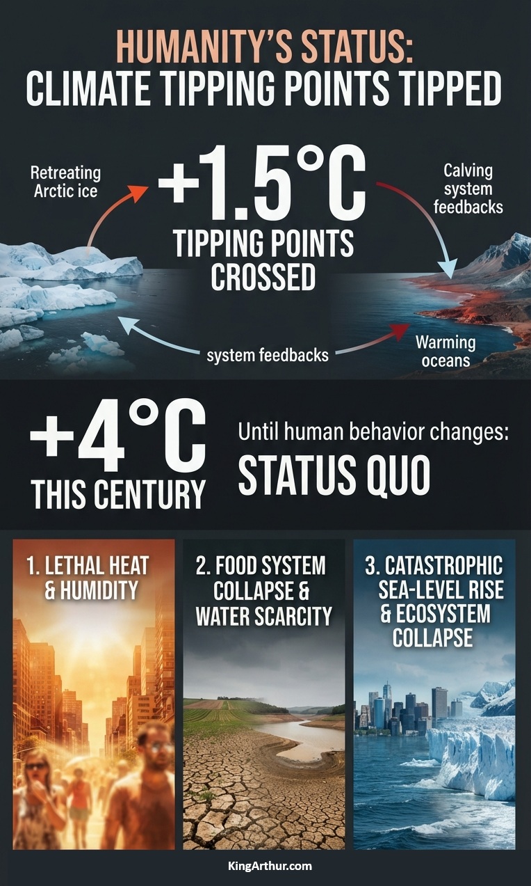
bookmark_borderHumanity’s Status: Climate Tipping Points Tipped

For now, until human behavior shows observable signs of change, the baseline trajectory remains “continued high emissions.” In addition, we have now crossed the 1.5°C threshold of self-reinforcing feedbacks and tipping points.

Under the status quo, human activities are most likely to push global average surface temperatures to +4°C this century.

The consequences include:

  1. Widespread Regional Uninhabitability via Lethal Heat and Humidity
  2. Collapse of the Global Food System and Severe Water Scarcity
  3. Irreversible Tipping Points: Catastrophic Sea-Level Rise and Ecosystem Collapse

https://www.kingarthur.com/global_warming

bookmark_borderRestricted Insurance Coverage Is Transmitting Climate Risk Through the Financial System

by Daniel Brouse and Sidd Mukherjee

Do you have homeowners insurance? If you answered yes, do you know what is actually covered when climate change and extreme weather damage your property?

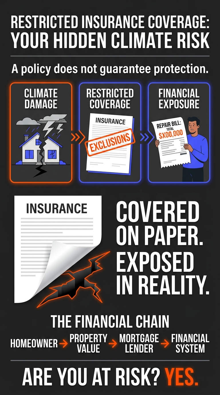
Most homeowners insurance policies exclude major categories of extreme weather damage, including flooding, while coverage for wind, hurricanes, and other hazards may be subject to significant limitations and exclusions. These restrictions are becoming more prevalent, creating one of the most significant emerging systemic risks to the global financial system.

In the United States, roof coverage is a particularly important concern. Many homeowners policies restrict roof-damage compensation through exclusions, depreciation provisions, actual-cash-value settlements, deductibles, or other limitations. Depending on the policy, a homeowner may have little chance of receiving enough compensation for a completely new roof, even when the damage is covered. As wind-related risks and losses intensify, these restrictions can leave homeowners responsible for an increasing share of repair and replacement costs.

The same principle applies to automobile insurance. If a tree is blown onto your car during a severe storm, are you covered? The answer depends on your policy, including whether you carry comprehensive coverage and whether any exclusions or limitations apply.

Climate change is already disrupting insurance markets, and the consequences extend far beyond rising premiums. Insurers are increasing prices, restricting coverage, declining renewals, and withdrawing from markets. These developments are creating growing financial vulnerabilities for homeowners, mortgage lenders, investors, businesses, and governments.

One of the most dangerous—and least understood—parts of this crisis is the expansion of restricted coverage. When an insurer refuses to cover a property, the problem is obvious. When a policy remains in force but excludes important risks, limits payouts, or imposes conditions that leave substantial losses uncovered, the danger is hidden. Homeowners may continue paying premiums believing they are protected, only to discover after a disaster that their policies do not cover the damage they suffered.

This is the delayed-disclosure trap: the financial vulnerability exists before the disaster, but its full consequences may not become apparent until a claim is denied or severely limited. By then, the homeowner may face repair costs, continuing mortgage obligations, and a damaged property without the insurance proceeds expected to cover the loss.

Restricted coverage can therefore undermine property values and mortgage security even when insurance remains available. A property may appear insured on paper while carrying substantial uninsured exposure. As these gaps widen, the distinction between having an insurance policy and having adequate financial protection has become increasingly important.

These developments are part of a larger system of interconnected feedbacks. Climate-related losses drive insurance costs higher and encourage insurers to limit their exposure. Higher costs and narrower protection weaken housing affordability and can depress property values. Declining property values and inadequate coverage increase financial risks for lenders and investors. When private insurance retreats, more costs shift to homeowners, businesses, and governments. These additional burdens can weaken the financial resources needed to prevent, withstand, and recover from future climate-related losses.

The central finding is that this feedback crisis is already underway. Rising premiums, insurance withdrawals, coverage restrictions, and growing exposure to uninsured losses are observable market developments. The interactions among these forces create additional risks that can reinforce one another, extending climate-related financial stress well beyond the locations directly affected by disasters.

The ultimate danger is not simply that insurance becomes more expensive. It is that insurance increasingly fails to provide the protection that households, lenders, and financial markets depend on. As this happens, climate risk has become a broader housing, credit, and economic crisis.

The Feedback Crisis Has Already Begun

The Whistleblower Warning: A Campaign to Expand Restricted Coverage

A memo by insurance-industry whistleblowers documents a disturbing development: the insurance industry is already well underway in what the whistleblowers characterize as a subversive campaign to expand restricted coverage, shifting financial risks onto homeowners without their full awareness.

The significance of this warning cannot be overstated. The expansion of restricted coverage changes the nature of the insurance crisis. The problem is no longer limited to rising premiums, canceled policies, or insurers refusing to cover high-risk properties. It also involves the erosion of protection within policies that homeowners continue to purchase and rely upon.

When insurers restrict coverage through exclusions, payout limitations, depreciation provisions, and other policy conditions, they can reduce their own exposure while transferring a greater share of potential losses to policyholders. When those restrictions are not adequately understood by homeowners, the transfer of risk can occur without a corresponding understanding of the financial consequences.

This creates a fundamental imbalance. Homeowners continue paying premiums and may reasonably believe they have protection against major property losses. Yet the actual terms of their policies may leave them responsible for substantial costs following a disaster. The gap between perceived protection and actual coverage can remain hidden until a claim is denied or the insurance payment falls far short of the amount needed to repair or replace damaged property.

The whistleblower warning therefore adds a critical dimension to the delayed-disclosure trap. Financial exposure is not simply increasing because climate-related disasters are becoming more costly. It is also increasing because the insurance protection intended to absorb those losses is being restricted, potentially without homeowners fully recognizing the changes.

The systemic consequences extend beyond individual households. Mortgage lenders may hold collateral whose owners cannot adequately insure or repair it. Investors may underestimate the uninsured exposure embedded in real estate portfolios. Communities may face declining property values and a growing burden of unrecoverable losses. When private insurance transfers more risk to homeowners, the resulting costs do not disappear. They are redistributed through household finances, mortgage markets, lending institutions, businesses, and ultimately, in some circumstances, governments and taxpayers.

This is the critical distinction: an insurance policy can remain active while the financial protection it provides deteriorates. Consequently, policy counts and insurance availability alone can understate the growth of climate-related financial risk.

The whistleblower allegations point to the need for scrutiny not only of insurance prices and market withdrawals, but also of how coverage restrictions are introduced, disclosed, and enforced. Regulators and policymakers must examine whether homeowners can readily understand the risks they are assuming, whether policy changes are adequately communicated, and whether the actual protection provided remains consistent with reasonable expectations.

If the documented practices are as extensive as the whistleblowers contend, the expansion of restricted coverage represents more than an insurance-market adjustment. It is a mechanism through which climate-related financial risk is being transferred to households while remaining largely concealed from homeowners, lenders, investors, and the broader financial system.

That makes restricted coverage a particularly dangerous link in the climate feedback crisis. The physical risk can increase, the financial protection can weaken, and the resulting vulnerability can remain hidden until a disaster exposes the full extent of the loss.

The Protection Gap Is a Critical Link in the Climate Feedback Crisis

The climate-insurance crisis is already unfolding. Rising premiums, restricted coverage, nonrenewals, and insurer withdrawals are changing the financial risks associated with property ownership. These are not merely forecasts of what might happen in a warmer future. They are observable developments whose economic consequences are already being felt.

Restricted coverage deserves particular attention because it can conceal financial exposure rather than eliminate it. When a policy excludes an increasingly important hazard, limits the amount payable, or imposes conditions that prevent a full recovery, the homeowner may remain exposed even while paying for insurance. The inadequacy of that protection may not become apparent until a disaster triggers a claim.

This delayed disclosure creates a dangerous mismatch between perceived security and actual financial resilience. Homeowners may believe their properties are protected. Mortgage lenders may assume that required insurance adequately safeguards their collateral. Investors may underestimate the exposure embedded in real estate portfolios. Yet a property with substantial uninsured risk can suffer serious financial damage even when an insurance policy remains active.

The consequences can reinforce one another. Climate-related damage increases insurance losses. Insurers respond through higher premiums, tighter policy terms, exclusions, and withdrawals. These changes increase ownership costs and expose homeowners to losses they cannot readily absorb. Property values and mortgage security can weaken, while financial distress, defaults, repair costs, and public financial obligations may rise. Governments and taxpayers can then inherit a larger share of the burden.

The feedback does not end there. When households, businesses, lenders, and governments must devote more resources to recovering from losses, fewer resources may remain available for risk reduction, resilience, and adaptation. If that shortfall leaves communities more vulnerable to subsequent disasters, future losses can grow, further intensifying insurance-market stress and financial instability.

This is the feedback mechanism at the heart of the crisis: climate risk increases financial vulnerability, and financial vulnerability is making society less capable of managing the next climate-related loss.

The appropriate response must therefore go beyond monitoring premiums and counting policy cancellations. Regulators, insurers, lenders, and policymakers need to examine what policies actually cover, how exclusions are changing, whether coverage limits remain adequate, and how much risk is being transferred to households and the public. Insurance availability alone is not a sufficient measure of financial protection.

The evidence establishes the need to take the observed disruption seriously and to investigate how its interacting effects are evolving. The precise scale and timing of future financial consequences remain uncertain, but the underlying feedback mechanisms are already visible. Waiting for the full consequences to emerge would mean waiting until hidden financial exposures become actual losses.

The critical question is no longer simply whether homeowners can obtain insurance. It is whether the insurance they can obtain will actually protect them when disaster strikes. As restricted coverage expands, the gap between insured property and adequately protected property has become one of the most consequential—and least visible—channels through which climate change destabilizes the economy.

Insurance can redistribute financial losses, but it cannot eliminate the physical risks that generate them. When those risks undermine the financial systems that support property ownership, lending, and investment, climate change becomes a systemic economic problem.

The insurance feedback crisis has already begun. Whether it remains manageable or develops into much broader financial instability depends on how quickly society recognizes these connections, exposes hidden coverage gaps, and acts to reduce the underlying risks.

bookmark_borderInsurance, Housing, Credit, and the Global Economy

by Daniel Brouse and Sidd Mukherjee

The Insurance Feedback Crisis: Climate Change Is Already Destabilizing Housing, Credit, and the Global Economy

How Rising Costs, Restricted Coverage, and Insurance Withdrawals Are Transmitting Climate Risk Through the Financial System

October 2026

Introduction

Climate change is already disrupting insurance markets, and the consequences extend far beyond rising premiums. Insurers are increasing prices, restricting coverage, declining renewals, and withdrawing from some markets. These developments are creating a growing financial vulnerability for homeowners, mortgage lenders, investors, businesses, and governments.

One of the most dangerous—and least understood—parts of this crisis is the expansion of restricted coverage. When an insurer refuses to cover a property, the problem is obvious. When a policy remains in force but excludes important risks, limits payouts, or imposes conditions that leave substantial losses uncovered, the danger is hidden. Homeowners may continue paying premiums believing they are protected, only to discover after a disaster that their policies do not cover the damage they suffered.

This is the delayed-disclosure trap: the financial vulnerability exists before the disaster, but its full consequences may not become apparent until a claim is denied or severely limited. By then, the homeowner may face repair costs, mortgage obligations, and a damaged property without the insurance proceeds expected to cover the loss.

Restricted coverage can therefore undermine property values and mortgage security even when insurance remains available. A property may appear insured on paper while carrying substantial uninsured exposure. As these gaps widen, the difference between having an insurance policy and having adequate financial protection becomes increasingly important.

These developments are part of a larger system of interconnected feedbacks. Climate-related losses drive insurance costs higher and encourage insurers to limit their exposure. Higher costs and narrower protection weaken housing affordability and property values. Reduced property values and inadequate coverage increase financial risks for lenders and investors. When private insurance retreats, more costs shift to homeowners, businesses, and governments. Those added burdens can weaken the financial resources needed to adapt to future climate risks.

The central finding is that this feedback crisis is already underway. Rising premiums, insurance withdrawals, coverage restrictions, and growing exposure to uninsured losses are observable market developments. The interactions among these forces are creating additional risks that can reinforce one another, extending climate-related financial stress well beyond the locations directly affected by disasters.

The ultimate danger is not simply that insurance becomes more expensive. It is that insurance increasingly fails to provide the protection that households, lenders, and financial markets depend on. When that happens, climate risk can become a broader housing, credit, and economic problem.

1. The Crisis Is Already Underway

For years, the economic consequences of climate change were discussed primarily in terms of future damage: projected disaster losses, future insurance costs, declining property values, and the possibility that some regions would eventually become uninsurable.

That framing is increasingly inadequate.

In vulnerable markets, insurance premiums have already risen sharply, coverage has become more restrictive, and some insurers have stopped writing new policies or withdrawn from particular areas. Property owners are confronting higher deductibles, policy nonrenewals, and fewer affordable alternatives. Public insurance programs have assumed greater importance in some jurisdictions where private coverage has become difficult to obtain.

These are present market developments, not merely projections.

Their significance extends beyond the insurance industry. Insurance is part of the financial infrastructure supporting property ownership, mortgage lending, commercial investment, and infrastructure development. When that infrastructure becomes more expensive or less accessible, the effects propagate into other sectors.

The emerging pattern is therefore not simply:

Climate change → More expensive disasters.

It is:

Climate change → Physical losses → Insurance disruption → Financial stress → Reduced economic resilience → Greater vulnerability to subsequent losses.

The final stages of this chain can feed back into the original problem. Households with fewer financial resources have less capacity to improve their properties. Municipalities under fiscal pressure have less flexibility to invest in protective infrastructure. Businesses facing higher insurance and borrowing costs may defer resilience investments.

The result is a system in which the costs of climate change can make society less capable of absorbing the next climate-related shock.

The insurance market is already exposing this vulnerability.

2. The Industry Is Warning About the Same Systemic Mechanism

The October 14, 2026, memorandum Sounding the Alarm, published by Inside Track x (Re)Insurance, describes concerns reported by senior professionals in the UK and European insurance, reinsurance, and brokerage sectors.

The memo identifies three principal responses to increasing physical risk:

  1. Higher premiums as insurers attempt to price expected losses and uncertainty.
  2. Restricted coverage as insurers narrow the risks they will accept.
  3. Market withdrawal when exposure cannot be made commercially viable.

All three responses are already familiar features of stressed insurance markets.

An insurer can reduce its own exposure by refusing to renew a policy. A reinsurer can protect its capital by increasing prices or reducing capacity. An underwriting department can improve its financial position by avoiding properties it considers too risky.

But none of these decisions removes the physical hazard.

Instead, the financial responsibility moves elsewhere. Homeowners retain more risk. Businesses absorb higher costs. Lenders face greater uncertainty about collateral. Governments confront greater pressure to support disaster recovery and provide insurance alternatives.

This creates a structural conflict between the financial stability of individual institutions and the financial stability of the broader economy.

The memo also warns that commercial incentives, limitations in catastrophe modeling, and fragmented assessments of exposure can prevent the industry from fully recognizing systemic risk.

The central warning reinforces an increasingly important conclusion: conventional risk management can protect individual institutions without adequately protecting the economic system in which they operate.

Restricted Coverage

Insurance is caught in a delayed-disclosure trap. When a homeowner cannot obtain coverage, the problem is immediately apparent. But an equally serious—and less visible—risk is the growing restriction of coverage. Policies may contain exclusions, limitations, and coverage gaps buried in the fine print, leaving homeowners exposed to losses they believe are insured. As insurers respond to rising risks and losses, these restrictions are expanding. The danger often becomes clear only after a disaster, when homeowners discover that their policies do not cover the damage. By then, it is too late to obtain the protection they thought they had.

3. The First Feedback Loop: Physical Losses Drive Insurance Disruption

The initial feedback begins with physical climate risk.

Flooding, wildfire, severe storms, extreme heat, and other hazards can damage buildings, interrupt businesses, destroy infrastructure, and increase claims. The consequences depend on the hazard, location, exposure, and vulnerability of the assets involved.

As insurers experience losses or revise their expectations of future losses, they adjust prices and coverage.

The initial sequence is direct:

Physical risk increases → Expected losses or uncertainty increase → Premiums rise and coverage tightens.

This relationship is already reflected in insurance-market decisions.

The feedback becomes more consequential when higher premiums and restricted coverage affect the financial viability of the properties being insured.

Insurance is not merely another household expense. It is part of the cost of maintaining property, satisfying mortgage requirements, operating a business, and attracting investment.

When insurance costs increase faster than household income or business revenue, the resulting financial pressure can become difficult to absorb. When suitable coverage disappears altogether, the problem changes from affordability to insurability.

The original physical risk has now produced a financial consequence that can persist even after a particular disaster ends.

A homeowner whose property survives a storm may still face a higher renewal premium. A business that escapes direct damage may still experience higher insurance costs. A community that avoids a catastrophic event may nevertheless face market repricing as insurers reassess its exposure.

This is the first critical transition: climate risk is no longer expressed exclusively through damage after a disaster. It is increasingly expressed through the cost and availability of financial protection before the next disaster occurs.

4. The Second Feedback Loop: Insurance Costs Pressure Property Values

Property values depend on more than a building’s physical condition and location. They also depend on the expected costs of ownership, the availability of financing, and the risks associated with future use.

Insurance disruption affects all three.

When premiums rise, the total cost of owning a property increases. When deductibles rise or coverage becomes less comprehensive, owners retain more potential financial loss. When insurers withdraw, buyers may have difficulty obtaining the coverage required by lenders or may have to accept more expensive alternatives.

These conditions can weaken demand for exposed properties.

The resulting feedback is:

Higher insurance costs → Higher ownership costs → Reduced affordability and buyer demand → Downward pressure on property values.

The process is already evident in the way insurance availability has become a growing consideration in real-estate transactions and property-risk assessments. Its magnitude varies by market, and a premium increase alone does not prove that property values have declined. But the economic mechanism is straightforward.

A property can lose economic value without suffering new physical damage. If buyers anticipate years of higher insurance costs, recurring flood losses, or difficulty obtaining a mortgage, they may be willing to pay less for it.

This creates a new form of climate-related financial exposure: the risk that the cost of protecting an asset undermines the value of owning it.

The implications are substantial because residential property represents a major share of household wealth. Commercial property supports business operations, employment, and investment. Property values also contribute to local tax revenues.

As insurance-related affordability problems spread, the consequences can extend beyond individual property owners into household balance sheets, commercial activity, and municipal finance.

5. The Third Feedback Loop: Property Risk Becomes Credit Risk

Mortgage lending depends on borrowers’ ability to repay their loans and on the value of the assets securing those loans.

Insurance supports both sides of that arrangement. It protects against specified losses that could impair collateral, while its premiums form part of the borrower’s ongoing cost of ownership. As insurance becomes more expensive or less available, both protections can weaken.

Higher premiums increase the monthly cost of homeownership. For financially constrained borrowers, that additional expense can reduce the ability to meet mortgage payments and other obligations. At the same time, inadequate coverage can leave a property owner and lender more exposed to the financial consequences of damage. If insurance difficulties reduce property demand or values, the collateral securing outstanding loans may also weaken.

The resulting feedback is:

Insurance disruption → Higher ownership costs and greater retained losses → Mortgage stress and weaker collateral → Increased credit risk.

The systemic concern is concentration. If insurance affordability deteriorates across a large number of properties in the same region, the financial consequences can occur together. Lenders may face correlated risks rather than isolated borrower problems. That possibility is particularly important where local economies, property tax revenues, employment, and household wealth are heavily dependent on real estate.

The risk is already being transmitted into financing decisions where insurance availability affects property transactions and underwriting. The connection between insurance and credit is established. The growing importance of climate-related insurability makes that connection increasingly consequential.

6. The Fourth Feedback Loop: Reinsurance Can Amplify Market Stress

Reinsurance provides financial protection to insurance companies against large or concentrated losses. It helps primary insurers manage their exposures and maintain the capacity to write policies. But reinsurance is itself exposed to catastrophe risk.

When reinsurers reassess expected losses or uncertainty, they may increase prices, change coverage terms, reduce available capacity, or require primary insurers to retain more risk. Primary insurers then face additional financial pressure. They may raise premiums, tighten underwriting, reduce policy limits, or withdraw from markets where acceptable returns cannot be achieved.

The feedback is:

Higher catastrophe losses or uncertainty → Reinsurance pressure → Higher primary-insurance costs or reduced capacity → Less affordable and less available coverage → Greater financial exposure outside the insurance system.

This process can spread the effects of physical risk beyond the location where a disaster occurs. An insurer’s response depends on its portfolio, reinsurance contracts, capital position, and exposure to multiple regions. The important point is that reinsurance does not eliminate catastrophe risk. It redistributes that risk through another layer of the financial system. If multiple insurers and reinsurers simultaneously reassess similar exposures, their decisions can reinforce market-wide tightening.

The October 2026 memo’s concern about interconnected risk is particularly relevant here. A firm may manage its own exposures prudently while the combined decisions of many firms reduce the capacity available to the wider economy.

The memo reinforces the need to monitor the relationship between physical losses, reinsurance costs, primary-market availability, and the financial resources available to absorb future losses.

7. The Fifth Feedback Loop: Public Intervention Transfers Costs to Taxpayers

As private insurance becomes unaffordable or unavailable, governments face growing pressure to intervene.

Public responses can include insurance programs of last resort, disaster assistance, infrastructure repairs, emergency housing, subsidized mitigation, and other forms of financial support.

Such measures can protect households and communities from immediate hardship. They can also preserve economic activity when private insurance capacity is insufficient. But they do not eliminate the physical losses. They redistribute part of the cost to public budgets.

The resulting feedback is:

Insurance withdrawal → Greater uninsured exposure → Increased demand for public support → Higher public expenditure and contingent liabilities → Greater fiscal pressure.

If the same communities repeatedly experience damaging events, governments may face recurring costs rather than a single temporary emergency. Meanwhile, the underlying economic base may weaken. Property values can come under pressure, businesses can suffer interruptions, and residents may relocate or reduce spending. These changes can reduce local revenues just as the need for public spending increases. The resulting fiscal squeeze is a direct consequence of the interaction between physical risk and financial vulnerability.

It is already visible in the expanding importance of public insurance and disaster-recovery arrangements in some exposed markets. The long-term fiscal consequences will depend on the scale of future losses, policy design, tax capacity, and the effectiveness of adaptation.

The danger is that public intervention can become a substitute for reducing underlying risk. If subsidies keep vulnerable properties insured without improving their resilience, governments may accumulate liabilities while leaving the physical exposure largely unchanged.

A sustainable response must therefore combine financial assistance with measures that reduce expected losses.

8. The Sixth Feedback Loop: Financial Stress Can Reduce Resilience

The preceding mechanisms reveal a more troubling feedback: the financial consequences of climate risk can reduce the capacity to manage future climate risk.

Consider a household facing higher premiums, a larger deductible, and rising repair costs. It may have less money available to install flood protection, replace a vulnerable roof, improve drainage, or strengthen the property against future damage.

Consider a municipality facing repeated disaster-recovery expenses and declining property revenues. It may have less capacity to upgrade stormwater infrastructure, maintain protective systems, or invest in long-term resilience.

Consider a business facing higher insurance and borrowing costs. It may delay investments that would otherwise reduce its exposure to future hazards.

The resulting feedback is:

Climate losses → Higher financial costs → Reduced capacity for adaptation → Greater vulnerability to subsequent losses.

This is a critical transition from a sequence of separate financial problems to a self-reinforcing system.

The original hazard creates damage or increases expected losses. Those losses generate financial pressure. Financial pressure constrains adaptation. Reduced adaptation leaves assets more exposed to future hazards. The next event then encounters a system that may be less prepared than before.

This mechanism is not merely theoretical. The financial constraints on households, municipalities, and businesses are real, and the need to pay for insurance and recovery competes with the need to invest in resilience.

9. The Combined Feedback System Is More Dangerous Than Any Individual Effect

The six feedbacks are interconnected.

Higher physical losses can raise insurance and reinsurance costs. Higher insurance costs can weaken property affordability. Reduced affordability can affect demand and financing. Weaker property values can increase credit risk and undermine local tax revenues. Public intervention can shift losses to taxpayers. Financial pressure can then reduce the resources available for adaptation.

These are not independent problems. They form a connected system in which stress in one sector can reinforce stress elsewhere.

The combined mechanism can be represented as follows:

Climate-related physical losses

↓

Higher insurance and reinsurance costs; restricted coverage and withdrawals

↓

Higher property ownership costs and greater uninsured exposure

↓

Weaker affordability, property demand, and financing conditions

↓

Increased mortgage vulnerability and public financial pressure

↓

Reduced resources for adaptation and recovery

↓

Greater vulnerability to future losses

The final step closes the feedback loop.

The significance is that the total economic effect can exceed the direct cost of any individual disaster. Financial interactions can prolong losses, transmit them to unaffected sectors, and weaken the capacity to recover. This is why insurance-market stress deserves attention as a systemic economic warning rather than simply an industry problem.

It also explains why waiting for an insurer or a major bank to fail would be the wrong approach. Financial instability can develop through declining affordability, reduced coverage, weaker investment, and growing public liabilities long before a dramatic institutional failure occurs.

The feedbacks do not need to culminate in a global financial collapse to cause substantial economic damage. They are already imposing persistent costs on households, businesses, and governments.

10. Why the 2008 Financial Crisis Is a Warning

The October 2026 industry memo compares the potential consequences of widespread uninsured property risk with vulnerabilities associated with the 2008 mortgage-market crisis. The comparison is useful because it highlights how problems involving property and credit can spread through interconnected financial relationships.

The 2008 crisis involved mortgage underwriting failures, excessive leverage, complex financial instruments, and weaknesses in financial oversight. Climate-related insurance disruption has a different underlying driver: changing physical risk and the difficulty of financing assets exposed to that risk.

The important similarity is the transmission mechanism. In both cases, problems involving the value, financing, or risk assessment of property can extend into lending and broader financial markets.

Climate-related insurance disruption can undermine property finance if coverage becomes unavailable, ownership costs rise sharply, or collateral values weaken. If these developments occur across many regions simultaneously, they could contribute to a broader financial shock.

The lesson is to recognize interconnected vulnerabilities before they become acute. Regulators and financial institutions should not wait for widespread defaults to begin evaluating how insurance-market disruption could affect lending, collateral, and public finance.

11. What the Evidence Already Shows

Observed developments

Insurance markets in several exposed regions are experiencing higher premiums, coverage restrictions, nonrenewals, and insurer withdrawals. Public insurance and disaster-assistance arrangements are increasingly important in some markets. Insurance availability is also an increasingly significant factor in property transactions and financial risk assessment.

These developments establish that insurance-market stress is already occurring.

Established economic mechanisms

Insurance costs affect property ownership expenses. Coverage requirements influence mortgage financing. Property values affect collateral. Reinsurance influences primary-market capacity. Public disaster spending affects government budgets.

These relationships provide a sound basis for evaluating how insurance disruption can transmit financial pressure across the economy.

Emerging systemic feedbacks

The interaction of insurance costs, property affordability, mortgage exposure, public liabilities, and reduced adaptation capacity creates a credible pathway toward self-reinforcing economic stress.

Uncertain outcomes

The crisis is already observable in its component parts. The systemic danger is that those parts can reinforce one another faster than institutions respond.

12. The Policy Response Must Address the Feedbacks, Not Just the Symptoms

The appropriate response is not simply to subsidize insurance premiums or require insurers to maintain coverage regardless of risk.

Those measures may provide temporary relief, but they cannot eliminate physical hazards. If they suppress risk signals without reducing exposure, they may encourage continued investment in vulnerable locations and transfer increasingly large liabilities to taxpayers.

A more effective response must address the causes and interactions of the feedback system.

Reduce the underlying physical risk

Greenhouse gas emissions influence long-term warming and many associated hazards. Reducing emissions limits additional future climate risk, although it cannot prevent all near-term losses.

Mitigation must be accompanied by adaptation because significant physical risks already exist.

Improve the resilience of exposed assets

Building standards, flood protection, drainage improvements, wildfire mitigation, resilient infrastructure, and risk-informed land use can reduce expected losses.

Investments should be evaluated against transparent estimates of their costs, benefits, maintenance requirements, and remaining exposure.

Where protection is not physically or economically sustainable, policymakers must consider fair and orderly relocation rather than assuming every property can be protected indefinitely.

Monitor the entire financial transmission chain

Regulators should examine insurance affordability and availability alongside mortgage performance, property values, reinsurance capacity, bank exposure, and public liabilities.

Stress tests should include scenarios in which insurance markets tighten across multiple regions at the same time.

The objective should be to identify correlated exposure before it generates substantial financial losses.

Improve catastrophe-model transparency

Insurers and reinsurers should clearly disclose material assumptions and uncertainties in their risk assessments. Independent review should investigate credible concerns about commercial pressure, inadequate data, and the underestimation of changing hazards.

The goal is to ensure that decisions reflect defensible estimates of risk rather than incentives to understate it.

Protect vulnerable households without concealing risk

Public support may be necessary to prevent immediate hardship and preserve access to essential coverage. But support should be linked, where appropriate, to mitigation, stronger building practices, and realistic assessments of long-term exposure.

A policy that preserves coverage without reducing the underlying risk defer costs rather than solve the problem.

13. Conclusion: The Feedback Crisis Has Already Begun

The Protection Gap Is a Critical Link in the Climate Feedback Crisis

The climate-insurance crisis is already unfolding. Rising premiums, restricted coverage, nonrenewals, and insurer withdrawals are changing the financial risks associated with owning property. These are not merely forecasts of what might happen in a warmer future. They are observable developments whose economic consequences are already being felt.

Restricted coverage deserves particular attention because it can conceal financial exposure rather than eliminate it. When a policy excludes an increasingly important hazard, limits the amount payable, or imposes conditions that prevent a full recovery, the homeowner may remain exposed even while paying for insurance. The inadequacy of that protection may not become apparent until a disaster triggers a claim.

This delayed disclosure creates a dangerous mismatch between perceived security and actual financial resilience. Homeowners may believe their properties are protected. Mortgage lenders may assume that required insurance adequately safeguards their collateral. Investors may underestimate the exposure embedded in real estate portfolios. Yet a property with substantial uninsured risk can suffer serious financial damage even when an insurance policy remains active.

The consequences can reinforce one another. Climate-related damage increases insurance losses. Insurers respond through higher premiums, tighter terms, exclusions, and withdrawals. Those changes increase ownership costs and expose homeowners to losses they cannot readily absorb. Property values and mortgage security can weaken, while defaults, repair costs, and public financial obligations may rise. Governments and taxpayers can then inherit a larger share of the burden. If these pressures reduce the resources available for prevention and adaptation, future losses can become even greater.

This is the feedback mechanism at the heart of the crisis: climate risk increases financial vulnerability, and financial vulnerability can make society less capable of managing the next climate-related loss.

The appropriate response must therefore go beyond monitoring premiums and counting policy cancellations. Regulators, insurers, lenders, and policymakers need to examine what policies actually cover, how exclusions are changing, whether coverage limits remain adequate, and how much risk is being transferred to households and the public. Insurance availability alone is not a sufficient measure of financial protection.

The evidence establishes the need to take the observed disruption seriously and to investigate how its interacting effects are evolving. The precise scale and timing of future financial consequences remain uncertain, but the underlying feedback mechanisms are already visible.

The critical question is no longer simply whether homeowners can obtain insurance. It is whether the insurance they can obtain will actually protect them when disaster strikes. As restricted coverage expands, the gap between insured property and adequately protected property may become one of the most consequential—and least visible—channels through which climate change destabilizes the economy.

Insurance can redistribute financial losses, but it cannot eliminate the physical risks that generate them. When those risks undermine the financial systems that support property ownership, lending, and investment, climate change becomes a systemic economic problem.

The feedback crisis has already begun. Whether it remains manageable or develops into much broader financial instability depends on how quickly society recognizes the connections and acts to reduce the underlying risks.


References and Further Reading

Primary industry source

Inside Track x (Re)Insurance. (October 14, 2026). Sounding the Alarm: Insurance and Reinsurance Memo.

https://static1.squarespace.com/static/697b3c8cf1bdde2c6ff1b5d5/t/6acebb5992f73c3954b746e5/1791933273139/Insurance+and+Reinsurance+Memo.pdf

This memo provides the principal industry perspective on physical risk, insurance repricing, coverage restrictions, market withdrawal, catastrophe modeling, and systemic financial vulnerability. Its findings should be interpreted in light of its aggregated and anonymized methodology.

Related research

Brouse, D., and Mukherjee, S. Climate Change and the Insurance Crisis: Rising Costs, Shrinking Availability, and the Limits of Insurability.

https://www.kingarthur.com/global_warming/Insurance-Cost-and-Availability.html

Brouse, D., and Mukherjee, S. Climate Change and Insurance: Costs, Availability, and Sustainability.

https://www.kingarthur.com/global_warming/Insurance-Cost-and-Availability-2025.html

Brouse, D., and Mukherjee, S. The Collapse Point: How Climate Change Is Breaking Insurance—and Capitalism With It.

https://www.kingarthur.com/global_warming/Insurance-Economic-Climate-Collapse.html

Brouse, D., and Mukherjee, S. Climate Risk, Insurance Market Instability, and Systemic Threats to Capital Formation.

https://www.kingarthur.com/global_warming/Insurance-Collapse-intro.html

Brouse, D. Financial Planning for Climate Change.

https://www.kingarthur.com/global_warming/Financial-Planning-for-Climate-Change.html

Brouse, D., and Mukherjee, S. Coupled Climate Feedbacks and Cascading Real Estate Risk.

https://www.kingarthur.com/global_warming/Feedbacks-Cascading-Real-Estate-Risk.html

Methodological note

This paper synthesizes an industry memorandum, related climate-insurance research, and established economic mechanisms. It does not present a new statistical model or independently estimate the probability of a global financial crisis. Claims about observed insurance-market disruption are distinct from claims about the magnitude of interconnected feedbacks or the timing of future systemic outcomes. Those latter questions require continued empirical investigation using insurance, reinsurance, property, credit, and public-finance data.

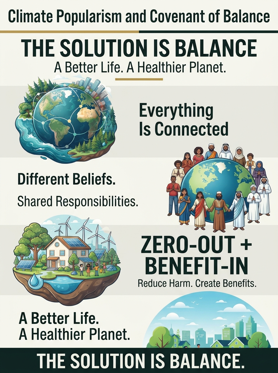
bookmark_borderThe Solution Is Balance: Making Climate Action Work for Everyone

A Practical Path to a Healthier Planet and a Better Life

Climate change is more than a problem of rising temperatures. It affects our homes, food supplies, health, economy, and the natural systems that support life. Addressing it requires science, practical solutions, shared values, and cooperation.

But there is a challenge: people are busy trying to make ends meet. They have bills to pay, families to support, and communities to protect. Climate action must address these everyday concerns if it is to gain lasting public support.

Two complementary ideas offer a way forward: Climate Popularism and the Covenant of Balance.

Start With What Matters to People

Climate Popularism, developed by Caroline Lucas and Rupert Read, argues that climate action should connect with the things people care about most.

Lower energy bills. Affordable food. Reliable transportation. Comfortable homes. Cleaner air and water. Safer communities.

These are not separate from climate action. Many practical improvements can help meet these needs while also reducing pollution and preparing communities for future risks.

For example, improving home insulation can reduce energy use and heating costs. Better public transportation can make travel more affordable. Protecting forests and restoring natural areas can support wildlife, protect water supplies, and help communities manage heat and flooding.

The goal is to make climate action useful in people’s daily lives.

What Does Balance Mean?

The Covenant of Balance builds on this practical approach by connecting climate science with shared ethical principles.

Earth is an interconnected system. The atmosphere, oceans, forests, soils, and living things all affect one another. Human life and our economy depend on these systems working well.

Climate change is one sign that this system is being pushed out of balance.

Earth receives energy from the Sun and releases energy back into space. Greenhouse gases from human activities trap additional heat, causing Earth’s climate system to gain energy. The oceans absorb most of this excess heat, while temperatures rise, ice melts, sea levels increase, and ecosystems change.

These effects can also interact. For example, when ice melts, darker surfaces are exposed. These surfaces absorb more sunlight, adding further warming.

Understanding these connections helps explain why reducing greenhouse gas emissions and protecting natural systems are both essential.

Balance does not mean that nature must never change. It means respecting the conditions that allow people and other living things to thrive.

Integrated Climate Stewardship: ZERO-OUT + BENEFIT-IN

Integrated Climate Stewardship’s guiding formula is simple:

ZERO-OUT + BENEFIT-IN

ZERO-OUT means reducing actual sources of harm. This includes cutting greenhouse gas emissions, wasting less energy, reducing pollution, and using fewer resources when doing so makes sense.

BENEFIT-IN means choosing improvements that also provide real benefits to people. These may include lower bills, better comfort, improved health, stronger local economies, and greater protection against extreme weather.

Consider a home that uses less energy for heating and cooling. The household may save money while also reducing pollution associated with energy use. A community that reduces food waste can save resources and lower disposal costs. A town that protects trees and improves stormwater management can create healthier neighborhoods while reducing certain local risks.

Not every project will produce every benefit. Costs, safety, local conditions, and actual environmental results must be considered.

The important point is to look for solutions that work in the real world.

Balance the Economy With the Environment

A healthy economy depends on healthy natural systems. Businesses need reliable supplies of water, energy, food, materials, and other resources. Communities need safe homes, functioning infrastructure, and a healthy population.

Economic growth that ignores environmental damage can create costs that others must eventually pay.

A better approach asks whether an activity meets a real need, whether it can be done with fewer resources, and whether its benefits justify its full costs.

This does not require rejecting markets, business, economic growth, or new technology. It means accounting for environmental damage rather than treating it as someone else’s problem.

Practical climate solutions should also consider fairness. Families with limited incomes may struggle to afford improvements even when those improvements would save money over time. Public programs, better financing, and community cooperation can help make effective solutions accessible to more people.

From Individual Action to Community Progress

Personal choices matter, but individual households cannot solve climate change by themselves.

Electricity generation, industry, transportation, agriculture, buildings, and public policy all play important roles. Businesses and governments must also reduce pollution and invest in practical improvements.

Communities can help by sharing useful information, improving public infrastructure, supporting vulnerable residents, and measuring progress openly.

The same standard should apply to everyone: look at the results.

Are emissions falling? Is energy being used more efficiently? Are costs manageable? Are communities becoming safer? Are natural systems being protected?

Good intentions are important, but measurable results are essential.

The Solution Is Balance

Climate Popularism offers a way to connect climate action with people’s everyday needs. The Covenant of Balance adds a broader ethical foundation, bringing together science, economics, environmental responsibility, and shared values.

Integrated Climate Stewardship provides the practical link between them: reduce actual harm while seeking measurable benefits for people and the planet.

We do not need to agree on every political, religious, or economic question to make progress. We need to recognize that our choices affect one another and that our long-term well-being depends on the natural systems that sustain us.

The goal is not to make people choose between a healthy planet and a better life.

The goal is to build a future in which protecting the planet helps people live healthier, safer, more affordable, and more fulfilling lives.

Different beliefs. Shared responsibilities. Practical solutions.

The solution is balance.


See:

Climate Popularism: https://assets.climatemajorityproject.com/Climate%20popularism%206Oct26.pdf

Covenant of Balance: https://www.kingarthur.com/global_warming/Covenant-of-Balance.html

bookmark_borderProducer Inflation Hits 6.3%, Highest Annual Rate Since December 2022

Yesterday’s consumer inflation report raised concerns about rising prices. Today’s producer inflation report delivered another unwelcome surprise, with wholesale prices rising far more than economists expected.

The U.S. Bureau of Labor Statistics released its September 2026 Producer Price Index (PPI) report on October 15, showing that wholesale prices jumped 1.3% for the month. That was the largest monthly increase since March 2022 and substantially exceeded economists’ forecast of 0.5%.

The annual producer inflation rate climbed to 6.3%, its highest level since December 2022.

Key Figures for September 2026

• Headline PPI (monthly): Rose 1.3%, compared with economists’ expectations of 0.5%.

• Headline PPI (annual): Increased 6.3% over the previous 12 months, the highest annual rate since December 2022.

• Final-demand goods: Jumped 2.6% for the month, driven largely by a 10.8% surge in energy prices. Gasoline prices climbed 20.3%.

• Final-demand services: Increased 0.8%, indicating that inflationary pressures extended beyond goods and energy.

• Core PPI (monthly): Rose 0.7%, excluding food and energy, more than double the expected 0.3% increase.

• Core PPI (annual): Reached 5.0%, suggesting that underlying producer-price pressures remain elevated even after volatile food and energy prices are excluded.

The Bottom Line

The September producer inflation report reinforces concerns that rising energy costs are spreading throughout the broader economy. Higher gasoline and energy prices increase transportation, shipping, manufacturing, and distribution costs. Businesses are already passing these higher costs along to consumers through increased prices for goods and services, as reflected in yesterday’s consumer inflation report.

This is the inflationary transmission mechanism at work: Higher production costs are rippling through supply chains, turning an initial energy-price shock into broader consumer inflation.

With annual producer inflation reaching 6.3% and core producer inflation hitting 5.0%, the pressure extends beyond the immediate impact of volatile energy prices. These figures indicate that businesses are facing substantial cost increases across the production chain, adding to inflationary pressure on consumer prices.

The critical question is whether September’s surge is temporary or marks the beginning of another broad-based inflationary wave. As higher production costs continue moving through the economy, consumers are facing increased prices for goods and services, even as the initial energy-price shock spreads beyond the energy sector.

Sources:

U.S. Bureau of Labor Statistics: https://www.bls.gov/ppi/

Barron’s: https://www.barrons.com/articles/ppi-inflation-report-september-producer-prices-6be6e2bb

bookmark_borderHow Is Climate Energy Hitting You? Biting: The Longest Mosquito Season

by Daniel Brouse

How Is Climate Energy Hitting You?

Biting: The Longest Mosquito Season

Southeastern Pennsylvania’s 2026 mosquito season has been prolonged, with mosquito activity extending into October. A combination of spring rainfall, warm temperatures, standing water, and persistent humidity can create favorable conditions for mosquito breeding and survival, potentially extending the season beyond its traditional peak.

The extended season is another example of how changing weather patterns can affect everyday life, from outdoor comfort to public health. However, confirming that 2026 is the region’s longest mosquito season would require historical surveillance data and consistent year-to-year comparisons.

The 2026 Mosquito Season: A Timeline

Early Start (April–May)

Warmer spring temperatures and rainfall can accelerate mosquito development and bring earlier seasonal activity. Standing water in yards, storm drains, and other locations provides breeding habitat. Establishing the precise start of the 2026 season requires local monitoring records.

Peak Season (June–August)

Summer heat can speed up mosquito development, while rainfall and persistent moisture can replenish breeding sites. Some mosquito species can complete their life cycle in as little as several days under favorable conditions. Urban drainage systems, containers, and low-lying areas can provide recurring sources of standing water.

Extended Autumn (September–October)

Mosquitoes can remain active well into autumn when temperatures and moisture levels remain favorable. Activity generally declines as temperatures fall, although the timing varies by species and local conditions. A hard frost can sharply reduce activity, but it does not necessarily eliminate all mosquitoes or their eggs.

Health Risks and Regional Hotspots

An extended mosquito season can prolong opportunities for exposure to mosquito-borne diseases, including West Nile virus (WNV). Actual risk, however, depends on local mosquito surveillance, virus detection, species distribution, and human exposure—not simply the length of the season.

The Vectors

Culex pipiens, commonly known as the northern house mosquito, is an important West Nile virus vector in Pennsylvania. It can thrive in urban environments, including storm drains and catch basins.

Aedes albopictus, the Asian tiger mosquito, is another important species in the region. It breeds in small collections of standing water, including water trapped in containers, and can remain active during suitable autumn weather.

West Nile Virus Surveillance

Pennsylvania and the Centers for Disease Control and Prevention monitor mosquito populations and mosquito-borne disease activity. Positive mosquito samples indicate that the virus is circulating in a particular area, but they do not, by themselves, establish the level of risk to residents.

Claims about early-season positive samples in Bucks County or other Southeastern Pennsylvania locations should be verified against the relevant 2026 surveillance records before publication.

What You Can Do

Residents can reduce mosquito breeding and exposure by taking a few practical steps:

  • Empty standing water from containers, flowerpots, buckets, and outdoor equipment.
  • Clean clogged gutters and maintain drainage around the property.
  • Use screens on windows and doors.
  • Apply an EPA-registered insect repellent according to its label.
  • Wear long sleeves and long pants when mosquitoes are active, particularly around dawn and dusk.

The Bottom Line

A longer mosquito season is more than an outdoor nuisance. It is a direct, increasingly visible consequence of a warming climate. Rising temperatures extend the period when mosquitoes can survive, reproduce, and remain active, pushing seasonal biting activity further into autumn and prolonging opportunities for exposure to mosquito-borne diseases.

Climate change is the primary long-term driver of warming temperatures and increasingly favorable conditions for extended mosquito seasons. Rainfall, humidity, standing water, mosquito species, and public-health interventions influence the severity of individual seasons, but a warming climate shifts the underlying conditions in favor of longer periods of mosquito activity.

The question is not just how much energy is accumulating in the climate system. It is how that energy translates into consequences we experience in our own backyards. In Southeastern Pennsylvania, a mosquito still biting in October offers a tangible reminder that climate change is not a distant threat. It is changing the conditions of everyday life—one bite at a time.

bookmark_borderTHE IMPACT OF TRUMPENOMICS

The U.S. Economy, Household Costs, Federal Debt, and America’s Global Economic Position

Comparative assessment: January 1, 2025 – October 12, 2026

1.Executive Summary

Since Donald Trump returned to office in January 2025, the United States has experienced a deteriorating mix of economic pressures: inflation has reaccelerated, long-term Treasury yields have risen sharply, mortgage rates remain near 7%, job growth has slowed, the trade deficit has widened, and household expenses continue to strain purchasing power. At the same time, federal deficits and debt-service costs remain exceptionally high, while the administration’s tariff strategy has generated legal and economic uncertainty. The boom in artificial intelligence (AI) and data-center construction has become an important source of capital spending, but it also drives demand for imported chips, servers, and other specialized equipment.

The administration emphasizes tax reductions, private-sector job creation, technology investment, and its claim that underlying inflation and real wages compare favorably with the Biden years. Those claims do not erase the impact of cumulative price increases, rising borrowing costs, and the deterioration in several key measures since the start of 2025. Taken together, the indicators examined here show an economy under significant pressure and raise serious questions about the results of Trumpenomics for ordinary households, productive investment, fiscal stability, and U.S. economic leadership.

2.1. Economic Performance Under Trump

GDP Growth: Promises Versus Results

An assessment of Trump’s economic record spans two distinct periods: his first term (2017–2021) and his second term (2025–present). From 2017 through 2019, before the pandemic, U.S. GDP grew at an average annual rate of approximately 2.5%. That was broadly comparable to the 2.3% average in the final three years of the Obama administration, but it fell short of Trump’s promise of sustained annual growth of 3% to 4%. In 2020, the COVID-19 pandemic caused GDP to contract by approximately 6.5% over his final year.

For the second term, the administration initially projected growth of 5% to 12%, yet the figures cited here put actual growth at roughly 2% annually, trailing the pace recorded during the latter half of the Biden administration. Real GDP growth slowed to 2.1% for 2025, compared with 2.8% in 2024, and the latest quarterly pace cited in this assessment has fallen to 0.7%. The contrast between ambitious growth promises and substantially weaker results is central to evaluating Trumpenomics.

Inflation and Interest Rates

Inflation remained low during much of Trump’s first term, hovering below the Federal Reserve’s 2% target. In the second term, that progress has stalled and reversed. By the end of 2025, year-over-year inflation had reached 2.7%; by autumn 2026, it had accelerated to approximately 3.5%–3.6%. Energy-price shocks have contributed to the renewed pressure, but they do not account for every source of inflation.

Treasury Secretary Scott Bessent’s October 9, 2026, “Trump Tracker” presents a more favorable interpretation, reporting annualized core inflation of 2.5% under Trump compared with 4.7% under Biden, and cumulative real weekly wage growth of 1.5%. Those measures are part of the administration’s case for its economic record. However, the broader household experience is also shaped by headline inflation and the cumulative rise in prices. Even when the rate of inflation slows, the price level generally does not return to where it stood before the increases.

The result is a continuing affordability crisis: groceries, housing, insurance, fuel, and borrowing remain expensive. The national gasoline average cited in this assessment has risen above $4.50 per gallon, while long-term borrowing costs have increased and mortgage rates remain near 7%. These conditions undermine the practical benefits of nominal wage gains for many households.

Labor Market and Employment

During Trump’s first term, the economy added roughly 7 million jobs before the pandemic downturn. In the second term, job creation has slowed sharply. The October 2026 figures cited here put average monthly job growth at approximately 27,000, reflecting a pullback in federal employment, restrictive immigration policies, and uncertainty associated with tariffs. The administration counters that it has added more than 1 million private-sector jobs while reducing the federal workforce by approximately 328,000 positions.

Both figures matter, but the distinction does not change the central concern: total employment growth has weakened considerably. A smaller federal workforce may reduce government payrolls, but it does not by itself demonstrate that the broader economy is creating enough jobs to support a growing labor force or offset the loss of public-sector positions.

3.2. Borrowing Costs: January 1, 2025, Compared with October 2026

The movement in benchmark interest rates reveals a tightening financial environment.

MetricJanuary 1, 2025October 2026Economic significance
10-year Treasury noteAbout 4.21%5.22%–5.24%Sharp increase, reflecting persistent inflation concerns and rising federal borrowing needs.

The 10-year Treasury yield has climbed to approximately 5.22%–5.24%, a level described in the underlying analysis as a 19-year high. Long-term yields can rise even when short-term rates fall because investors are pricing in persistent inflation, heavier government borrowing, and uncertainty about the long-run fiscal outlook. Mortgage rates remain structurally close to 7%, worsening affordability for buyers and adding to the cost of housing across the economy.

4.3. Tax Policy, Federal Deficits, and National Debt

Tax Cuts and Distributional Effects

Trump’s first term produced the $3.2 trillion Tax Cuts and Jobs Act, while his second term enacted the One Big Beautiful Bill Act (OBBBA). The administration describes these measures as historic tax cuts for working Americans. The Institute on Taxation and Economic Policy (ITEP), however, finds that the benefits disproportionately favor the wealthiest 1%, with an average tax cut exceeding $70,000 for the top tier. By contrast, the bottom 20% face minor tax increases under the cited analysis because of restrictions on credits.

The distribution of tax benefits is therefore a central measure of the policy’s economic impact. A tax cut’s headline size does not establish that it improves the financial position of most households, especially when the benefits are concentrated among high-income taxpayers and households continue to face rising costs for essential goods and services.

Deficit Growth and Debt-Service Costs

The federal deficit has expanded to approximately 6% of GDP, and the Congressional Budget Office projects that it will approach 7% by 2033. The fiscal-year 2026 deficit is estimated at $1.99 trillion, a 12% increase from the prior year and the largest annual gap since 2021. Net interest payments are consuming approximately 3.3% of U.S. GDP, placing a growing burden on the federal budget.

The national debt continues to compound beyond the $34–$35 trillion range cited in the original analysis, while debt held by the public is approximately 100% of GDP. Long-term projections indicate that, without substantial fiscal changes, publicly held debt could rise to 175% of GDP over the next three decades. As Treasury yields rise, refinancing and new borrowing become more expensive, further increasing interest costs and constraining future budget choices.

5.4. Tariffs, Trade Policy, and Legal Reversals

Trump’s “America First” strategy relies heavily on protectionist tariffs to shield domestic industries, encourage U.S. manufacturing, and reshape international trade. During his first term, he replaced NAFTA with the USMCA and initiated a trade war with China. The second-term tariff program has created additional uncertainty for manufacturers, importers, retailers, and consumers.

Tariffs raise the cost of imported goods and industrial inputs, creating upward pressure on prices and disrupting supply chains. They may benefit some protected domestic producers, but those benefits come with costs to businesses that depend on imported components and to consumers who face higher prices. The resulting uncertainty can also discourage investment when firms cannot reliably predict future input costs or market access.

The administration initially presented tariff revenue as a major source of funding that could offset tax cuts and reduce federal obligations. In fiscal year 2025, customs duties temporarily surged by 250% to approximately $195 billion. Nonpartisan estimates indicated that, if maintained permanently, the tariffs could reduce the cumulative ten-year deficit by $3 trillion.

That strategy encountered a major legal obstacle in early 2026, when the U.S. Supreme Court ruled that the administration had exceeded its authority by using the International Emergency Economic Powers Act (IEEPA) to impose broad global tariffs. The resulting legal reversal undermined the administration’s original revenue projections. The analysis estimates that the loss of the broader tariff authorities created a $200 billion–$250 billion budget hole and caused customs-duty projections to fall by 60%. With narrower mechanisms remaining, the applied tariff rate is estimated at approximately 11.8%.

The tariff burden on households remains substantial. The Tax Foundation estimates cited here put the average household cost of the initial full-scale tariffs at approximately $1,000 in 2025 and the cost under the post-ruling tariff structure at approximately $820 annually. Tariffs have therefore failed to deliver a straightforward path to eliminating the trade deficit or reducing household costs.

6.5. Inflation, Producer Costs, and the Trade Deficit

Consumer and Producer Prices

The Consumer Price Index (CPI) measures changes in the prices paid by consumers, while the Producer Price Index (PPI) tracks changes in prices received by domestic producers. The draft’s comparison shows CPI inflation rising from approximately 2.5% in early 2025 to 3.5%–3.6% by autumn 2026. Producer costs have also risen, driven by industrial-component constraints, grid-modernization expenses, and supply-chain pressures. These increases put pressure on businesses before costs are passed through to households.

Trade Deficit

The monthly trade deficit stood at approximately $96.8 billion at the start of 2025 and has widened to a reported record of $105.6 billion. This outcome runs counter to the administration’s stated goal of using import taxes to eliminate the trade gap. A major factor is the surge in imports of capital goods, including semiconductors and advanced computing equipment needed to build AI infrastructure.

The trade balance reflects more than tariff rates alone. It is shaped by domestic saving and investment, exchange rates, consumer demand, business investment, and the availability of goods from overseas. In this period, the rapid construction of data centers has increased demand for specialized chips, servers, and other technology components that U.S. suppliers cannot immediately provide at the required scale.

7.6. AI, Data Centers, and the Composition of GDP Growth

AI infrastructure is one of the defining features of the second Trump administration’s economic platform. The administration claims to have attracted more than $2.7 trillion in technology and AI investment to preserve U.S. technological dominance. AI and data-center construction have become a major source of capital spending even as broader GDP growth has slowed.

The figures cited here estimate that compute-infrastructure capital expenditure has doubled from its historical baseline and now represents approximately 0.8% of U.S. GDP. Total data-center and technology-infrastructure spending is estimated at approximately 1.5% of GDP. These investments support construction, electrical equipment, cooling, networking, and advanced computing, but they also require large quantities of imported semiconductors and specialized hardware.

This creates an important tension in the headline numbers: AI investment supports measured economic activity, while its imported components widen the trade deficit. The growth of AI infrastructure should not be mistaken for uniformly strong performance across the entire economy. The composition of GDP matters, as do the domestic value added, productivity gains, and long-term returns produced by these investments.

8.7. Household Costs: Fuel, Food, Insurance, and Taxes

Gasoline and Diesel

Regular gasoline was below $3.50 per gallon in early 2025. The national average cited here has since risen by 27.4% over the past year, exceeding $4.50 per gallon. Diesel has moved from below $4 per gallon to nearly $6 nationally, with prices exceeding $8 in parts of California. Disruptions affecting transport through the Strait of Hormuz have intensified pressure on fuel markets and raised costs across freight, agriculture, manufacturing, and household transportation.

Beef and Produce

Food prices reflect years of accumulated increases as well as current supply pressures. Since 2020, beef roasts have risen approximately 73%, steaks 57%, and standard ground beef 52%, with prices continuing to climb through 2026. Fruit and vegetable prices have increased more slowly—approximately 2.2% year over year in the cited data—but remain at historically high levels. Fertilizer, labor, refrigeration, transport, and other input costs continue to affect the price of produce.

Homeowners Insurance and Total Household Taxes

The national annual homeowners-insurance baseline cited for 2025 was approximately $2,912. For older properties, the later average is estimated at $3,086, an increase of roughly 6% in one year. Insurance costs add to the financial burden of homeownership, alongside elevated mortgage rates, maintenance costs, and property taxes.

The tax burden must be evaluated across federal, state, and local levels, including property taxes. The OBBBA’s federal tax changes provide substantial benefits to high-income households under the cited ITEP analysis, while credit restrictions leave the bottom 20% facing minor tax increases. Meanwhile, local property taxes have risen as municipalities seek revenue for infrastructure and public services. Federal tax cuts do not necessarily translate into lower total household taxes when local taxes and other mandatory expenses are rising.

Real Wages and Other Significant Costs

The cited data show real average hourly earnings declining by 0.3% over the past year. That means inflation has outpaced nominal wage gains over the period measured, reducing purchasing power. The administration’s reported 1.5% cumulative increase in real weekly wages uses a different measure and comparison window; it does not eliminate the pressure created by higher accumulated prices.

Other costs are adding to the squeeze. Non-mortgage credit defaults have reached multi-decade highs, and subprime auto-loan delinquencies have risen to 6.9%, exceeding the peak recorded during the 2008 financial crisis according to the figures cited here. High vehicle prices and elevated annual percentage rates (APRs) make financing increasingly expensive. Rent, utilities, medical care, childcare, and revolving consumer debt further constrain household budgets.

9.8. Federal Fiscal Pressure and the Cost of Capital

The U.S. faces a highly constrained fiscal landscape in which large deficits, a growing debt stock, and higher interest rates reinforce one another. Treasury yields have risen as investors price in persistent inflation and the long-term consequences of federal borrowing. Higher yields raise the government’s cost of capital and can also increase financing costs for households and businesses.

The tariff program was presented as a way to generate revenue, offset tax cuts, and reduce national obligations. But the legal reversal of broad tariff authority weakened those projections, while tariffs themselves raised costs for American households and firms. The original fiscal rationale has therefore collided with legal limits, higher consumer costs, and a trade deficit that has continued to widen.

10.9. How the Pressures Interact

The economic pressures are connected rather than isolated. Expanding deficits and defense spending increase Treasury borrowing needs and can push yields higher. Higher yields raise the cost of government debt, mortgages, and business financing. Tariffs and supply-chain disruptions raise input prices, while AI and data-center construction increase imports of specialized computing hardware. A stronger dollar can make imports less expensive but can also make U.S. exports less competitive, while overseas demand for AI hardware can increase import volumes.

Expanding deficits and defense spending → Higher Treasury yields → Higher financing costs
AI and data-center demand → More imported semiconductors and equipment → Wider trade deficit
Tariffs and supply-chain disruption → Higher input costs → Greater consumer-price pressure
Combined effects → Household strain, investment uncertainty, and weaker long-term fiscal flexibility

11.Conclusion: The Economic Record of Trumpenomics

The economic record since January 1, 2025, is marked by renewed inflation pressure, higher long-term Treasury yields, mortgage rates near 7%, sharply slower job creation, a widening trade deficit, and continued increases in essential household expenses. At the same time, tax cuts have disproportionately benefited the wealthiest households under the cited distributional analysis, federal deficits remain above 6% of GDP, and interest payments consume an increasing share of national output.

The administration points to private-sector job gains, AI investment, and favorable measures of core inflation and real weekly wages. Yet those indicators must be considered alongside the full economic picture: cumulative price increases, household fuel and food costs, homeowners insurance, property taxes, credit distress, and the rising cost of borrowing. Announced investment is not the same as broad-based prosperity, and tariff revenue has not eliminated the trade deficit or insulated consumers from higher costs.

The combined evidence presents a troubling assessment of Trumpenomics. The policies have intensified uncertainty across trade and supply chains, left the federal government facing large deficits and growing debt-service costs, and failed to resolve the affordability pressures confronting American households. AI investment offers a significant source of technological and economic opportunity, but its contribution should be measured against its import requirements and the broader economy’s performance—not used to obscure weaknesses elsewhere.

12.Principal Measures Referenced

GDP growth: approximately 2.5% average annual growth in 2017–2019; 2.1% in 2025; latest quarterly pace cited at 0.7%.

Inflation: approximately 2.7% at the end of 2025 and 3.5%–3.6% by autumn 2026; administration-reported annualized core inflation of 2.5%.

Employment: approximately 27,000 average monthly jobs added in the cited October 2026 data; administration-reported 1 million private-sector jobs added and 328,000 federal positions reduced.

Borrowing costs: 10-year Treasury 4.21% to 5.22%–5.24%

Federal finances: fiscal-year 2026 deficit approximately $1.99 trillion; deficit above 6% of GDP; net interest approximately 3.3% of GDP.

Trade: monthly deficit approximately $96.8 billion at the start of 2025 versus a reported $105.6 billion later in 2026.

Household costs: gasoline above $4.50 per gallon; diesel near $6 nationally; substantial cumulative beef-price increases; homeowners insurance rising approximately 6%.

AI infrastructure: compute capex estimated at 0.8% of GDP; broader data-center and technology infrastructure spending estimated at 1.5% of GDP.

bookmark_borderINTEGRATED CLIMATE FEEDBACK (Alternative Version)

by Daniel Brouse

INTEGRATED CLIMATE FEEDBACK, COUPLING, AND TIPPING-POINT NETWORK

POLAR AMPLIFICATION, CRYOSPHERE, AND ICE-SHEET NETWORK

POLAR AMPLIFICATION → Arctic warming exceeding the global average → weakened equator-to-pole temperature gradients → changes in atmospheric circulation, storm tracks, and polar jet-stream dynamics → accelerated Arctic sea-ice loss + Greenland ice melt → changes in surface albedo, ocean heat exchange, freshwater input, and atmospheric stability →

ICE–ALBEDO FEEDBACK: sea-ice + snow + land-ice loss → darker ocean + land surfaces exposed → reduced surface albedo → greater absorption of incoming solar radiation during sunlit periods → additional surface warming → further ice + snow loss ↺

MELT–ELEVATION FEEDBACK: Greenland + ice-sheet surface melting → reduced ice-sheet elevation → exposure of the ice surface to warmer atmospheric conditions at lower elevations → faster surface melt → further elevation loss ↺

REGIONAL LAPSE-RATE FEEDBACK: Arctic warming → changes in the vertical atmospheric temperature gradient and atmospheric stability → altered vertical temperature contrasts + near-surface radiative cooling → enhanced near-surface warming under favorable polar conditions → additional sea-ice and surface-ice loss ↺

ARCTIC OCEAN HEAT STORAGE–WINTER SEA-ICE FEEDBACK: Arctic sea-ice loss → increased summer solar absorption by open water → increased upper-ocean heat storage → autumn + winter ocean-to-atmosphere heat release → delayed freeze-up + reduced winter sea-ice growth → further sea-ice loss ↺

COUPLED CRYOSPHERIC AMPLIFICATION: sea-ice loss + snow retreat + glacier and ice-sheet melting + permafrost thaw → reduced surface reflectivity + changes in land and ocean heat exchange + freshwater input + altered ground hydrology → atmospheric circulation changes + ocean stratification changes + additional cryospheric stress →

SNOW–ALBEDO FEEDBACK: warming → reduced snow cover + earlier seasonal snowmelt → darker land surface exposed → reduced reflectivity → increased solar absorption → additional land-surface warming → further snow loss ↺

GLACIAL-RETREAT FEEDBACK: atmospheric warming + ocean heat reaching glacier fronts → surface melting + submarine melting in susceptible regions → glacier retreat + ice discharge → changes in ice-surface elevation + local albedo + freshwater input → additional cryospheric and oceanic changes ↺ → SEA-LEVEL RISE → coastal inundation + erosion + saltwater intrusion + altered coastal ecosystems + infrastructure stress + changes in coastal carbon storage → increased environmental and socioeconomic vulnerability →

EXTREME PRECIPITATION–CRYOSPHERE FEEDBACK: warming → increased atmospheric moisture capacity + changes in precipitation intensity, phase, and seasonal distribution → altered snowfall accumulation + rain-on-snow events + surface-meltwater delivery → changes in glacier and ice-sheet mass balance + runoff + basal hydrology → changes in ice accumulation or loss → further cryospheric change ↺

WEST ANTARCTIC ICE-SHEET TIPPING ELEMENT: ocean warming + basal ice-shelf melting → ice-shelf thinning → reduced buttressing in susceptible regions → increased grounded-glacier discharge → potential marine ice-sheet instability → persistent ice loss + sea-level rise → additional coastal and cryospheric stress →

ICE-SHEET MELT–COASTAL CARBON CROSS-LINK: ice-sheet mass loss → sea-level rise → coastal flooding + erosion + saltwater intrusion → changes in wetlands, marshes, mangroves, and other coastal ecosystems → possible loss of stored carbon + reduced future sequestration → additional atmospheric CO₂ relative to a healthy-ecosystem baseline → increased greenhouse forcing where net carbon storage declines ↺

WILDFIRE–SNOW AND ICE-ALBEDO CROSS-LINK: wildfire emissions → black-carbon deposition on snow + ice → reduced reflectivity → increased solar absorption → accelerated snowmelt + glacier melt → greater exposure of darker surfaces → further absorption of solar energy ↺

BOREAL FOREST–SNOW–ALBEDO COUNTEREFFECT: boreal forest loss → increased snow exposure during snow-covered seasons → increased surface reflectivity → potential regional cooling that partially offsets greenhouse warming. At the same time, forest loss → reduced carbon storage + altered evapotranspiration + changes in surface roughness + potentially greater fire susceptibility → additional warming or ecosystem stress. Net effect depends on latitude, season, snow cover, forest type, and the balance of biogeophysical and carbon-cycle effects.

PERMAFROST–FIRE–DEEPER THAW CROSS-LINK: warming + drying → increased fire susceptibility in some permafrost landscapes → wildfire → combustion of vegetation + loss of insulating organic layers → altered ground thermal properties + deeper seasonal thaw → increased exposure of frozen organic carbon to decomposition → CO₂ + CH₄ emissions under suitable conditions → additional greenhouse forcing → further warming and thaw ↺

EARTH MASS REDISTRIBUTION–ROTATION CONNECTION: global land-ice loss + redistribution of terrestrial water and ice mass → changes in Earth’s moment of inertia + angular momentum distribution → small changes in Earth’s rotation rate, length of day, and polar motion. Groundwater depletion and redistribution also affect Earth’s mass distribution and rotation. These are geophysical consequences of mass redistribution, not independent climate feedbacks.

OCEAN HEAT CONTENT, STRATIFICATION, CARBON, AND CIRCULATION NETWORK

PLANETARY ENERGY IMBALANCE–OCEAN HEAT CONTENT: planetary energy imbalance → accumulation of excess heat in the Earth system, with the ocean absorbing the majority of the excess energy → increased ocean heat content (OHC) → changes in ocean temperature, vertical heat distribution, circulation, and ocean–atmosphere exchange → altered regional climate and cryospheric conditions →

OCEAN HEAT VARIABLES—DISTINCT BUT COUPLED: ocean heat content → total heat stored throughout the ocean; sea-surface temperature → surface conditions governing evaporation, convection, and air–sea exchange; vertical mixing + stratification → redistribution of heat between surface and deeper waters; ocean–atmosphere heat exchange → transfer of heat between ocean and atmosphere. These variables interact but are not interchangeable: increasing OHC does not require uniform surface warming or uniform warming at every depth.

ALBEDO–CLOUD–OCEAN HEAT CONTENT TRIAD: low-level cloud decline in regions and seasons where clouds exert a net cooling effect → reduced reflection of incoming shortwave solar radiation → increased absorbed solar energy → increased ocean heat uptake + OHC → ocean warming → changes in atmospheric moisture + stability + circulation → further low-level cloud decline where conditions favor the response ↺

OHC–CRYOSPHERE FEEDBACK: OHC ↑ → ocean warming + changes in vertical heat distribution → increased subsurface heat exposure to marine-terminating glaciers or ice shelves in susceptible regions → basal ice melting + ice discharge → freshwater input + ice loss → changes in ocean stratification + surface albedo → further oceanic and cryospheric changes ↺

OCEAN STRATIFICATION–MARINE HEATWAVE FEEDBACK: surface ocean warming + freshwater input → stronger upper-ocean stratification under favorable conditions → altered vertical mixing and heat redistribution → increased persistence of elevated upper-ocean temperatures in susceptible regions → marine heatwaves + ecosystem stress → changes in marine carbon uptake + air–sea heat exchange → additional regional ocean changes, with feedback direction dependent on local conditions ↺

NORTH ATLANTIC STRATIFICATION–GLACIER-FRONT HEAT FEEDBACK: Greenland meltwater + changes in precipitation and evaporation → upper-ocean freshening + altered stratification → changes in deep convection, mixing, and ocean heat redistribution → regionally altered subsurface heat delivery to marine-terminating glacier fronts where circulation permits → changes in basal melting + ice discharge → additional freshwater input ↺

OHC–AMOC FEEDBACK: OHC ↑ + changes in freshwater input + density structure + wind forcing + ocean mixing → changes in North Atlantic stratification and deep convection → potential AMOC weakening + altered ocean heat transport → regional redistribution of ocean heat → changes in subsurface heat exposure + atmospheric heat exchange + moisture transport → further oceanic, atmospheric, and cryospheric changes ↺

AMOC–CIRCULATION CROSS-LINK: AMOC changes → altered North Atlantic and hemispheric heat distribution → changes in ocean–atmosphere heat exchange + atmospheric temperature gradients → potential changes in Northern Hemisphere storm tracks, regional precipitation, and circulation → changes in Greenland melt + Arctic sea ice + freshwater distribution → further ocean and atmospheric responses. The strength and direction of the response are regionally dependent; AMOC weakening does not establish that collapse is inevitable.

AMOC–CLOUD FEEDBACK: AMOC changes → North Atlantic sea-surface temperature + circulation changes → altered moisture transport + atmospheric stability → changes in low-level cloud formation, altitude, thickness, and persistence → changes in shortwave reflection + longwave trapping → regional changes in absorbed energy → further ocean warming or cooling and potential AMOC stress, depending on the net radiative response ↺

AMOC–ICE-MELT FEEDBACK: AMOC changes → altered North Atlantic heat transport → regional ocean–atmosphere temperature redistribution → changes in Greenland + Arctic ice melt → freshwater discharge → changes in North Atlantic surface salinity + density → changes in deep-water formation and overturning circulation → potential additional AMOC weakening ↺

AMOC–STRATIFICATION–OCEAN CARBON FEEDBACK: AMOC changes + ocean warming + stratification changes → altered ventilation + nutrient transport + carbon redistribution → changes in ocean CO₂ uptake and storage → changes in atmospheric CO₂ relative to an alternative circulation scenario → altered greenhouse forcing → further ocean and atmospheric changes where net effects reinforce the original change ↺

OCEAN CARBON SINK–CIRCULATION FEEDBACK: ocean warming + stratification + circulation changes → altered CO₂ solubility + ventilation + nutrient supply + biological carbon export → changes in ocean carbon uptake and storage → changes in atmospheric CO₂ → altered radiative forcing → further climate and ocean changes ↺. The ocean remains a major carbon sink; uptake changes in magnitude and distribution rather than necessarily stopping.

OCEAN OXYGEN–ECOSYSTEM–CARBON FEEDBACK: ocean warming + stratification → reduced oxygen supply to subsurface waters in susceptible regions → deoxygenation + changes in nutrient cycling + marine ecosystem stress → altered biological carbon export + carbon storage + greenhouse-gas production in some environments → changes in ocean–atmosphere carbon exchange → additional climate forcing where net effects reinforce warming ↺

TROPICAL OCEAN VARIABILITY–GLOBAL CIRCULATION NETWORK: ENSO + other tropical ocean variability → changes in tropical sea-surface temperature patterns + convection → changes in atmospheric heating + pressure patterns + moisture transport → shifts in planetary waves, jet streams, monsoons, and storm tracks → changes in regional heat + rainfall + drought + wildfire conditions → changes in land and ocean energy, water, and carbon exchanges → further regional climate responses. Greenhouse warming changes the background conditions on which natural variability operates.

TROPICAL CIRCULATION–CLOUD–OCEAN HEAT FEEDBACK: tropical ocean warming patterns → changes in convection + atmospheric circulation + moisture transport → changes in cloud distribution + altitude + persistence + reflectivity → altered shortwave absorption + longwave trapping → changes in regional solar absorption + ocean-surface heating → changes in sea-surface temperature gradients + tropical circulation → further cloud and ocean-heat redistribution ↺

OHC–ATMOSPHERIC INSTABILITY–LIGHTNING NETWORK: ocean warming + changes in atmospheric moisture and convection → changes in convective instability in susceptible regions → changes in lightning activity → lightning-generated nitrogen oxides (NOₓ) → increased tropospheric ozone formation under suitable chemical and meteorological conditions → vegetation damage → changes in carbon uptake + evapotranspiration → changes in atmospheric moisture + clouds → altered radiation and regional climate forcing.

LOW-LEVEL CLOUDS, WATER VAPOR, AEROSOLS, AND RADIATION NETWORK

LOW-LEVEL CLOUD–OCEAN HEAT FEEDBACK: low-level cloud cover ↓ in regions and seasons where clouds exert a net cooling effect → reflected shortwave radiation ↓ → absorbed solar energy ↑ → ocean heat uptake + OHC ↑ → ocean warming + changes in atmospheric stability and moisture → changes in cloud formation + persistence → further cloud decline where the response reinforces the initial change ↺

CLOUD SHORTWAVE–LONGWAVE RADIATION BALANCE: changes in cloud cover + altitude + thickness + droplet properties + geographic distribution → changes in reflected incoming shortwave sunlight + absorption and emission of outgoing longwave radiation → changes in net cloud radiative effect → changes in planetary energy balance and regional temperatures. Low clouds often cool by reflecting sunlight; high clouds can warm by trapping outgoing infrared radiation. The net effect depends on cloud type, location, altitude, optical thickness, season, and underlying surface.

LOW-LEVEL CLOUD DECLINE–ARCTIC AMPLIFICATION CROSS-LINK: low-level cloud decline during periods and in regions where clouds have a net cooling effect → increased solar energy reaching the surface → enhanced surface and ocean warming → sea-ice loss + reduced albedo → Arctic amplification → changes in atmospheric stability + moisture + circulation → further changes in cloud formation. During polar night and cold seasons, low clouds can exert a warming effect through longwave trapping; cloud decline does not produce uniform warming in all conditions.

ATMOSPHERIC WATER-VAPOR FEEDBACK: warming → increased atmospheric water vapor where moisture is available → increased absorption of outgoing infrared radiation → stronger greenhouse trapping → additional warming → increased atmospheric moisture capacity + changes in evaporation → further water-vapor increases where moisture supply permits ↺. Water vapor is primarily a feedback on warming, while long-lived greenhouse gases are major external drivers.

AEROSOL–CLOUD–RADIATION COUPLING: wildfire smoke + industrial pollution + changing biogenic emissions + other aerosols → altered aerosol abundance + composition + particle properties → changes in cloud-droplet formation + cloud lifetime + reflectivity + precipitation → altered shortwave and longwave radiation → regional warming or cooling + hydrological changes → further vegetation stress and fire risk under favorable conditions ↺

AEROSOL COOLING COUNTEREFFECT: certain anthropogenic aerosols + volcanic aerosols → scattering or reflection of sunlight and, for some aerosols, cloud-brightening effects → reduced incoming solar energy reaching the surface → temporary cooling that partially offsets greenhouse-gas warming. Aerosol effects vary by composition, altitude, location, and cloud interactions; cooling effects do not remove the health and environmental harms of air pollution.

LOW-LEVEL CLOUD–OZONE COUPLING: tropospheric ozone → vegetation damage + altered stomatal function → changes in transpiration and surface moisture → changes in boundary-layer development + atmospheric humidity + low-level cloud formation → changes in shortwave reflection + longwave trapping → regional warming or cooling depending on cloud response → changes in ozone chemistry and vegetation stress under suitable conditions ↺

AMOC–OZONE FEEDBACK: AMOC changes + altered atmospheric circulation → changes in atmospheric chemistry + ozone-precursor transport → changes in tropospheric ozone formation and distribution → vegetation damage → reduced photosynthesis and altered stomatal conductance → changes in evapotranspiration + atmospheric moisture → changes in low-level cloud formation → altered radiation where cloud properties change → additional regional warming or cooling and possible further ocean stress. Each link is conditional on local chemistry and meteorology.

OZONE–CARBON SINK FEEDBACK: tropospheric ozone → plant injury + reduced photosynthesis and, in sensitive vegetation, altered stomatal function → reduced terrestrial carbon uptake relative to a healthier-vegetation baseline → greater atmospheric CO₂ retention → increased greenhouse forcing → additional warming → further vegetation stress and possible carbon-sink degradation under favorable conditions ↺

ATMOSPHERIC CIRCULATION, JET STREAM, AND EXTREME WEATHER NETWORK

JET-STREAM COUPLING: Arctic amplification + changes in tropical heating + stratospheric conditions + internal variability → changes in meridional temperature gradients and atmospheric circulation → changes in polar jet-stream structure + Rossby-wave propagation + storm tracks → possible changes in jet-stream waviness, progression, and blocking → persistent weather patterns in susceptible configurations → heat extremes + drought + heavy precipitation + stalled atmospheric rivers → hydroclimatic whiplash → agricultural + infrastructure + ecosystem + public-health stress → increased vegetation stress and wildfire risk → further land–atmosphere changes ↺. The effects vary by region, season, and circulation regime.

SOIL MOISTURE–EVAPOTRANSPIRATION–HEAT FEEDBACK: warming → soil drying where precipitation and water supply are insufficient → reduced soil moisture availability → reduced evaporation + plant transpiration → reduced evaporative cooling + increased sensible heat flux → higher land-surface and near-surface air temperatures → increased atmospheric moisture demand → further soil drying ↺ → increased risk of heat extremes + drought + vegetation stress + wildfire.

LAND–ATMOSPHERE DROUGHT COUPLING: prolonged heat + reduced precipitation → declining soil moisture → reduced evapotranspiration → increased near-surface sensible heating + atmospheric moisture demand → boundary-layer changes + reduced local moisture recycling → greater heat and drought stress where circulation and moisture supply reinforce the response ↺

VEGETATION–ROUGHNESS–CIRCULATION FEEDBACK: forest loss + canopy degradation → changes in surface roughness + albedo + energy and water exchange → changes in boundary-layer mixing + atmospheric stability + cloud formation + rainfall → additional heat and moisture stress where the response is reinforcing → further vegetation degradation ↺

WILDFIRE–CLOUD FEEDBACK: wildfire smoke + vegetation loss → altered aerosol loading + surface energy balance + moisture flux → changes in cloud formation + persistence → altered shortwave reflection + longwave trapping → regional warming or cooling depending on aerosol and cloud properties → precipitation disruption in susceptible conditions → greater drought and fire risk where conditions reinforce the cycle ↺

EXTREME PRECIPITATION–SOIL MOISTURE CROSS-LINK: warming → changes in atmospheric moisture capacity and precipitation extremes → intense rainfall and flooding in some regions + longer dry intervals in others → changes in soil-water storage, runoff, erosion, vegetation condition, and groundwater recharge → altered drought and flood vulnerability → further land–atmosphere and ecosystem impacts.

WILDFIRE, LIGHTNING, AND ATMOSPHERIC CHEMISTRY NETWORK

WILDFIRE–OZONE FEEDBACK: warming + drought → increased wildfire risk under conducive weather and fuel conditions → vegetation loss + smoke + atmospheric emissions → increased ozone precursors → tropospheric ozone formation under suitable chemical conditions → vegetation damage → reduced carbon uptake and changes in evapotranspiration → greater warming and drying relative to a healthier-ecosystem baseline → increased wildfire risk ↺

LIGHTNING–OZONE FEEDBACK: warming + changes in convective instability → changes in lightning frequency and intensity → lightning-generated NOₓ → increased tropospheric ozone formation under suitable chemical conditions → vegetation damage → changes in carbon uptake and evapotranspiration → further ecosystem and climate stress → changes in future lightning potential. The pathway depends on storm type, moisture, background chemistry, and atmospheric transport.

LIGHTNING–WILDFIRE FEEDBACK: warming + drying → increased fuel flammability in susceptible ecosystems → lightning ignition → wildfire → vegetation loss + carbon emissions + changes in surface energy balance → additional warming and drying where net effects reinforce the initial conditions → greater wildfire risk ↺

FIRE–CARBON–SOIL FEEDBACK: warming + drought → wildfire → vegetation loss + soil-carbon combustion + post-fire decomposition → reduced ecosystem carbon storage + altered soil structure + moisture retention → reduced regeneration + increased surface heating + greater fuel vulnerability → additional carbon release and wildfire susceptibility ↺

AEROSOL–FIRE–PRECIPITATION COUPLING: wildfire emissions → changes in aerosol properties + cloud microphysics + atmospheric heating → changes in cloud development + precipitation efficiency + regional circulation → altered drought and fuel-moisture conditions → further wildfire risk under favorable conditions ↺

WILDFIRE AEROSOL–SNOW/ICE CROSS-LINK: wildfire smoke → aerosols in the atmosphere → changes in incoming solar radiation + cloud microphysics, with possible short-term cooling or warming depending on conditions. Separately, black-carbon deposition on snow and ice → reduced albedo → increased solar absorption → accelerated melting. Atmospheric smoke effects and deposited soot effects must be distinguished.

LAND CARBON, FORESTS, VEGETATION, AND ECOSYSTEM FEEDBACK NETWORK

CARBON-SINK DEGRADATION NETWORK: tropospheric ozone + warming + drought + wildfire + land-use change → reduced vegetation productivity and photosynthesis + increased carbon release in affected ecosystems → declining terrestrial carbon uptake relative to a healthier-ecosystem baseline → more atmospheric CO₂ retained → increased greenhouse forcing → additional warming → stronger ecosystem stress → further carbon-sink degradation where the response reinforces the initial change ↺

LAND CARBON SINK–ATMOSPHERIC CO₂ FEEDBACK: heat + drought + ozone damage + wildfire + ecosystem degradation → reduced photosynthesis and carbon storage, plus increased respiration or combustion emissions in some conditions → atmospheric CO₂ accumulation relative to a healthier-ecosystem baseline → increased radiative forcing → additional warming → greater ecosystem stress ↺. Land ecosystems can continue to absorb carbon where conditions remain favorable.

BOREAL FOREST TIPPING ELEMENT: warming + drought + wildfire + ozone damage + insect and disease stress → forest degradation and possible persistent forest transition → reduced carbon uptake + increased carbon release in affected systems → changes in albedo + snow exposure + evapotranspiration + surface roughness → regional cooling through snow exposure in some seasons, but potential warming through carbon loss and hydrological changes → further forest stress where net effects reinforce degradation ↺

AMAZON RAINFOREST TIPPING ELEMENT: warming + drought + fire + ozone damage → reduced plant function + photosynthesis + evapotranspiration in susceptible areas → reduced rainfall recycling and changes in cloud formation → increased drought stress where moisture recycling weakens → forest degradation + possible persistent forest loss → reduced carbon storage + carbon release → additional warming → further forest stress ↺. The extent of this pathway depends on regional rainfall, land use, fire, ecosystem resilience, and future climate.

VEGETATION–MOISTURE–CLOUD FEEDBACK: vegetation damage + forest loss → changes in transpiration + moisture recycling → changes in atmospheric humidity + cloud formation + rainfall → increased regional heat and drought stress where moisture recycling weakens → additional vegetation damage ↺. In other settings, cloud and rainfall responses may differ.

VEGETATION–OZONE–FIRE COUPLING: ozone damage + drought → reduced plant productivity and altered stomatal function → reduced carbon uptake + changes in evapotranspiration → greater atmospheric CO₂ retention and reduced evaporative cooling under susceptible conditions → increased heat and drought stress → greater wildfire susceptibility → further vegetation loss + carbon emissions ↺

OZONE–SOIL MOISTURE–HEAT EXTREMES CROSS-LINK: ozone exposure → plant injury + altered stomatal conductance and transpiration → changes in soil-water use and surface energy partitioning → potentially reduced evaporative cooling + increased sensible heating → greater risk of local heat extremes under susceptible conditions → additional plant stress. Reduced transpiration can conserve soil water in some circumstances, so the net soil-moisture response depends on species, rooting depth, soil, and weather.

PERMAFROST, WETLANDS, AND METHANE NETWORK

PERMAFROST TIPPING ELEMENT: Arctic warming → permafrost thaw → exposure of previously frozen organic matter to decomposition → release of CO₂ + CH₄ under suitable conditions → additional greenhouse forcing → further warming → additional permafrost thaw ↺

PERMAFROST HYDROLOGY–THERMOKARST FEEDBACK: Arctic warming → permafrost thaw + ground-ice loss → ground subsidence + thermokarst formation → altered drainage + wetland formation or drying → changes in soil moisture, oxygen availability, and anaerobic conditions → altered soil-carbon decomposition + CO₂ and CH₄ emissions → additional greenhouse forcing → further permafrost thaw ↺. Thaw can make some landscapes wetter and others drier.

WETLAND–METHANE FEEDBACK: warming + altered precipitation + permafrost thaw → changes in wetland extent + water-table depth + anaerobic conditions → changes in microbial methane production and emissions → changes in atmospheric CH₄ → altered greenhouse forcing → further warming → additional wetland and permafrost changes ↺. Regional drying can reduce methane emissions while increasing CO₂ emissions from drained organic soils.

PERMAFROST–FIRE–CARBON FEEDBACK: Arctic + boreal warming → drying vegetation + increased fire susceptibility in some landscapes → wildfire → combustion of vegetation + exposed soil organic carbon → reduced surface insulation + altered ground thermal properties → deeper seasonal thaw + additional carbon release → further warming and ecosystem stress ↺

COUNTERACTING AND STABILIZING CLIMATE RESPONSES

PLANCK RESPONSE: surface and atmospheric warming → increased outgoing longwave infrared radiation → greater energy loss to space → a stabilizing negative feedback that opposes the initial warming, without necessarily offsetting the full forcing from increased greenhouse-gas concentrations.

CONDITIONAL LOW-CLOUD COUNTERFEEDBACK: changes in circulation + atmospheric stability + moisture + aerosols → increased low-level cloud cover in some regions or seasons → increased reflection of incoming sunlight → reduced local or regional solar energy absorption. The net effect depends on the cloud’s longwave trapping, altitude, thickness, location, and season.

SNOWFALL AND ICE-ACCUMULATION COUNTEREFFECT: increased atmospheric moisture in some cold regions → increased snowfall where temperatures and precipitation conditions permit → temporary increases in snow accumulation or glacier and ice-sheet mass → partial offset of surface-melt losses. The net mass balance still depends on melt, rain-on-snow, and ice discharge.

AEROSOL COOLING COUNTEREFFECT: certain anthropogenic and volcanic aerosols → scattering or reflection of sunlight + possible cloud-brightening effects → reduced solar energy reaching the surface → temporary cooling that partially offsets greenhouse warming. The effect varies with aerosol composition, altitude, location, and cloud interactions.

CONTINUING TERRESTRIAL AND OCEAN CARBON UPTAKE: plant growth + terrestrial ecosystem recovery + ocean carbon uptake → removal of some atmospheric CO₂ → partial moderation of greenhouse-gas accumulation. Uptake depends on ecosystem health, nutrient and water availability, ocean chemistry, temperature, and circulation; neither terrestrial nor oceanic uptake should be assumed to cease universally.

COUNTERACTING FEEDBACKS ARE NOT PROOF OF CLIMATE STABILIZATION: negative feedbacks and regional cooling effects operate alongside reinforcing feedbacks and external forcing. The net climate trajectory depends on their relative magnitude, timing, geographical distribution, and interaction with human emissions.

EXTERNAL FORCING, FEEDBACK, TIPPING ELEMENTS, AND IMPACTS

EXTERNAL AND ANTHROPOGENIC FORCING: greenhouse-gas emissions → increased absorption of outgoing infrared radiation → planetary energy imbalance → atmospheric + land + ocean warming. Additional forcings include anthropogenic aerosols, land-use change, and natural solar and volcanic variability, each with distinct effects on the climate system.

REINFORCING FEEDBACKS: warming or another initial disturbance → changes in water vapor, cloud radiative effects, albedo, ocean circulation, soil moisture, or carbon storage → additional change in the original direction where the net feedback is positive ↺

COUNTERACTING FEEDBACKS: warming or another disturbance → changes that oppose the original disturbance, including increased outgoing infrared radiation and certain regional cloud, aerosol, or snow responses → partial stabilization or redistribution of energy.

TIPPING ELEMENTS: Greenland and Antarctic ice sheets + Arctic sea ice + AMOC + permafrost carbon stores + boreal forests + Amazon rainforest → components that may undergo substantial persistent change if particular thresholds are crossed. Thresholds, reversibility, confidence, and timescales differ by system; not every feedback is a tipping point.

CLIMATE CONSEQUENCES AND IMPACTS: persistent warming + changes in circulation, hydrology, cryosphere, and ecosystems → sea-level rise + extreme heat + drought + heavy precipitation + wildfire + agricultural stress + ecosystem disruption + infrastructure damage + water insecurity → economic + migration + public-health + political stress.

SOCIETAL–ENVIRONMENTAL CROSS-LINK: climate-related food + water + infrastructure + economic stress → changes in migration, public policy, land use, and resource demand → potential changes in emissions, ecosystem protection, and vulnerability → further environmental and societal consequences. These effects depend on human choices, institutions, adaptation, and resilience; they are not an inevitable one-way cascade.

INTEGRATED DOMINO EFFECT AND SYSTEM-WIDE COUPLING

ARCTIC WARMING → polar amplification → changes in equator-to-pole temperature gradients and atmospheric circulation → changes in weather persistence and regional extremes → drought + wildfire + vegetation stress in susceptible regions → altered carbon sinks + evapotranspiration → changes in clouds + atmospheric chemistry → changes in planetary energy balance → further warming where net effects reinforce the initial change ↺

OCEAN WARMING → OHC ↑ → changes in surface temperature + vertical heat redistribution + stratification + air–sea heat exchange → marine heatwaves + glacier-front melting + altered circulation → potential AMOC stress + changes in clouds and ocean carbon storage → changes in regional albedo + absorbed solar energy + atmospheric CO₂ → further ocean and atmospheric changes where net effects reinforce the initial disturbance ↺

VEGETATION DAMAGE → ozone + drought + wildfire + land-use change → photosynthesis and carbon uptake ↓ in affected ecosystems + changes in evapotranspiration → atmospheric CO₂ retention ↑ relative to a healthier-ecosystem baseline + changes in atmospheric moisture → warming + cloud changes → drought and fire risk ↑ in susceptible regions → further vegetation damage ↺

ICE LOSS → albedo changes + freshwater discharge ↑ + sea level ↑ → regional energy redistribution + ocean stratification and circulation changes + coastal ecosystem stress → additional cryospheric, hydrological, and ecological changes where feedbacks reinforce the initial disturbance ↺

ATMOSPHERIC CHEMISTRY–ECOSYSTEM COUPLING: greenhouse gases + ozone precursors + aerosols + wildfire emissions → changes in radiative forcing + plant function + cloud microphysics → altered carbon sinks + hydrological processes + atmospheric circulation → additional climate-system changes. The net response depends on chemical conditions, aerosol properties, cloud type, and ecosystem sensitivity.

GLOBAL CARBON–ENERGY COUPLING: terrestrial carbon-sink changes + ocean carbon uptake changes → changes in atmospheric greenhouse-gas concentrations relative to a baseline → changes in radiative forcing → further warming → additional ecosystem + ocean stress → further changes in carbon uptake and storage where net effects reinforce the initial change ↺

INTEGRATED DOMINO EFFECT: climate warming → feedback activation or modification → feedback coupling → nonlinear amplification or counteraction → possible threshold approach or crossing → potential tipping-element destabilization → cascading Earth-system changes → food + water + infrastructure + economic + migration + political stress → additional environmental and societal vulnerability.

OVERARCHING DYNAMICAL SEQUENCE

ENERGY IMBALANCE → HEAT REDISTRIBUTION → FEEDBACK ACTIVATION → FEEDBACK COUPLING → AMPLIFICATION OR COUNTERACTION → THRESHOLD APPROACH → POSSIBLE THRESHOLD CROSSING → POTENTIAL TIPPING-ELEMENT DESTABILIZATION → CASCADING SYSTEM RESPONSE → FURTHER CHANGES IN ENERGY, WATER, AND CARBON FLOWS ↺

TIMESCALE CLASSIFICATION

FAST ATMOSPHERIC PROCESSES: cloud formation and changes, water-vapor responses, aerosol–radiation interactions, atmospheric chemistry, lightning, storms, and many heat extremes → response over days to years, depending on the mechanism.

INTERMEDIATE OCEAN–LAND–ECOSYSTEM PROCESSES: upper-ocean heat redistribution, marine heatwaves, soil-moisture feedbacks, regional circulation changes, forest stress, wildfire recovery, and changes in carbon uptake → response over seasons to decades or longer.

SLOW AND THRESHOLD-SENSITIVE PROCESSES: deep-ocean adjustment, large ice-sheet retreat, long-term sea-level rise, permafrost carbon release, and persistent forest or ecosystem transitions → response over decades to centuries or longer, with some changes potentially persisting for millennia.

CROSS-SCALE COUPLING: fast atmospheric responses → changes in intermediate ocean, land, and ecosystem processes → potential activation of slow or threshold-sensitive responses → long-lasting changes that can influence the atmosphere and ocean well before the slow component has fully adjusted.

Interpretive principle: A reinforcing pathway indicates the potential for amplification, not proof of inevitability. A tipping element requires evidence of threshold-sensitive behavior, and a coupled network must be assessed link by link. The central systems question is how energy, water, and carbon move through the Earth system—and whether their interactions strengthen, weaken, or persist as conditions change.