High-Risk U.S. Real Estate Regions Under the Multiplicative Climate Risk Framework

Posted on 2026/08/082026/08/08 by admin

by Daniel Brouse and Sidd Mukherjee

The Multiplicative Climate Risk Formula

The Multiplicative Climate Risk Formula is a real-estate climate-risk model designed to capture how multiple hazards and vulnerabilities can interact and compound rather than occur independently. The framework incorporates interconnected risks including sea-level rise, storm surge, extreme precipitation, flooding, hydroclimatic whiplash, wildfires, drought, extreme heat, hurricanes, landslides, avalanches, and other cascading hazards.

Rather than treating each hazard as an isolated threat, the model evaluates how hazard exposure, hazard coupling, structural vulnerability, insurance stress, and recovery deficits can multiply overall real-estate risk.

The central premise is simple:

Climate risk is not merely additive. When multiple vulnerabilities interact, their combined impact can be substantially greater than the sum of their individual effects.

Applying the Multiplicative Climate Risk Formula reveals an important characteristic of climate-driven real-estate risk: the highest-risk regions are not necessarily those experiencing the most dramatic individual weather events. The greatest systemic risk emerges where multiple risk dimensions interact and amplify one another.

A region can experience severe hurricanes, wildfires, flooding, or extreme heat without necessarily experiencing the highest level of cascading real-estate risk. The critical question is what happens when physical hazards interact with high exposure, hazard coupling, structural vulnerability, insurance-market stress, and limited recovery capacity.

The framework therefore evaluates five interacting dimensions:

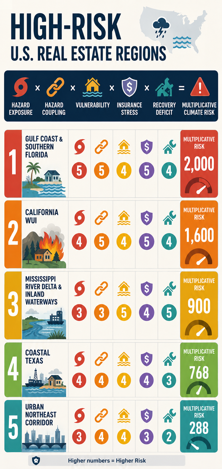
Hazard Exposure × Hazard Coupling × Vulnerability × Insurance Stress × Recovery Deficit = Multiplicative Climate Risk

Each component is scored from 1 to 5, where:

1 = Low Risk

2 = Moderate-Low Risk

3 = Moderate Risk

4 = High Risk

5 = Extreme Risk

The resulting score is not a probability of loss or a conventional actuarial measure. It is a comparative systems-risk index designed to identify locations where multiple weaknesses can reinforce one another.

This distinction is critical.

A region with a score of 5 in one category but relatively low scores elsewhere may be less systemically exposed than a region scoring 4 or 5 across nearly every category.

The multiplicative framework captures that interaction:

Physical Hazard ↑ + Coupling ↑ + Vulnerability ↑ + Insurance Stress ↑ + Recovery Capacity ↓ → Cascading Real-Estate Risk ↑↑

The following ranking represents a comparative assessment of major U.S. real-estate risk regions, incorporating physical hazards and the increasingly important financial and institutional dimensions of climate exposure.

1. Gulf Coast & Southern Florida

The Compound-Compounding Zone

Hazard Exposure — 5/5

The Gulf Coast and southern Florida face some of the country’s most concentrated combinations of acute and chronic climate hazards.

These include:

Major Hurricanes + Storm Surge + Extreme Rainfall + Sea-Level Rise + Coastal Flooding + Extreme Heat

The region’s vulnerability is not based on any single hazard. It is the convergence of multiple hazards affecting a densely developed coastal real-estate market.

Hazard Coupling — 5/5

The defining characteristic is the interaction among hazards.

A tropical cyclone can simultaneously produce:

Storm Surge + Extreme Rainfall + River Flooding + High Winds

Sea-level rise increases the baseline upon which storm surge occurs, while extreme rainfall can overwhelm drainage systems at the same time that elevated coastal water levels restrict drainage.

The resulting process is:

Hurricane → Storm Surge + Extreme Rainfall → Drainage Impairment → Compound Flooding → Widespread Property Exposure

This is precisely the type of coupled hazard that can produce disproportionate economic consequences.

Vulnerability — 4/5

The region contains enormous quantities of residential, condominium, commercial, and infrastructure assets exposed to coastal and flood hazards.

Building age and construction standards vary substantially. Newer construction and mitigation measures can reduce vulnerability, while older structures and properties with inadequate flood, wind, or drainage protection remain substantially more exposed.

The critical issue is therefore not simply the age of the housing stock, but the mismatch between:

Long-Lived Real Estate Assets → Rapidly Changing Climate Risk

Insurance Stress — 5/5

Insurance is one of the most consequential real-estate constraints in the region.

The combination of hurricanes, storm surge, flooding, wind damage, sea-level rise, and repeated catastrophe losses places substantial pressure on insurance availability and affordability.

The resulting feedback is:

Climate Risk ↑ → Expected Losses ↑ → Insurance Premiums ↑ → Deductibles and Coverage Restrictions ↑ → Insurance Availability ↓

For homeowners, insurance costs directly increase the cost of ownership.

For commercial real estate, rising insurance expenses can reduce net operating income and asset values by increasing operating costs. The effect is particularly significant for multifamily, hospitality, retail, and other income-producing properties.

The insurance problem therefore extends beyond individual policies.

It becomes a real-estate valuation problem:

Insurance Cost ↑ → Cost of Ownership ↑ → Buyer Demand ↓ → Property Values ↓

Recovery Deficit — 4/5

The region’s substantial public and private capital resources provide recovery capacity, but the scale of the infrastructure challenge is enormous.

Long-term pressures include:

Flood-Control Systems + Pump Stations + Drainage Networks + Seawalls + Roads + Bridges + Utilities + Wastewater Systems

The concern is not whether these systems can recover from one disaster.

The concern is whether:

Repeated Damage > Available Recovery and Adaptation Capacity

If the frequency of major events increases faster than infrastructure can be repaired, upgraded, or relocated, a recovery deficit can develop.

Multiplicative Risk

5 × 5 × 4 × 5 × 4 = 2,000

Total Risk Factor: 2,000

The Gulf Coast and southern Florida therefore represent the most pronounced example of compound climate-real-estate risk in the framework.

2. Central & Southern California Wildland-Urban Interface

The Fire–Flood–Insurance Cascade Zone

Hazard Exposure — 4/5

The Central and Southern California WUI faces a combination of:

Wildfire + Extreme Heat + Drought + Water Stress + Extreme Rainfall

The exposure is particularly consequential because enormous quantities of residential real estate have been constructed adjacent to or within wildfire-prone landscapes.

Hazard Coupling — 5/5

The defining feedback is:

Drought → Vegetation Stress → Wildfire → Vegetation Loss → Soil Destabilization → Extreme Rainfall → Mudslides and Debris Flows

This is a classic sequential compound-risk mechanism.

Wildfire does not simply produce immediate property losses.

It can alter the landscape in ways that increase the consequences of subsequent precipitation events.

The result is:

Wildfire → Landscape Transformation → Increased Post-Fire Flood/Mudslide Risk

This creates a risk cascade extending beyond the original fire.

Vulnerability — 4/5

Residential development in steep terrain, narrow canyons, and areas with constrained evacuation routes can create substantial exposure.

Vulnerability also depends on construction standards, defensible space, vegetation management, access routes, and the ability of communities to recover rapidly after catastrophic fires.

Insurance Stress — 5/5

California represents one of the clearest examples of insurance-market stress becoming a real-estate problem.

The combination of catastrophic wildfire exposure, rapidly changing risk conditions, and repeated losses creates pressure on insurers to increase premiums, restrict coverage, reduce exposure, or withdraw from high-risk markets.

When private insurance becomes unavailable or unaffordable, property owners may be forced into residual or state-backed insurance mechanisms.

The resulting feedback is:

Wildfire Risk ↑ → Insurance Losses ↑ → Premiums ↑ → Coverage Restrictions ↑ → Private Insurance Availability ↓ → Residual-Market Dependence ↑

This creates a second real-estate feedback:

Insurance Availability ↓ → Financing Constraints ↑ → Buyer Pool ↓ → Property Liquidity ↓ → Property Values ↓

The insurance problem can therefore become a leading indicator of broader real-estate repricing.

Recovery Deficit — 4/5

Large wildfire events can produce extensive reconstruction requirements simultaneously.

The recovery system must contend with:

Destroyed Housing + Infrastructure Damage + Debris Removal + Labor Requirements + Construction Demand + Supply Constraints

The resulting competition for labor and materials can extend rebuilding timelines and increase reconstruction costs.

The longer recovery takes, the greater the potential for:

Recovery Delay → Business Interruption → Household Displacement → Reduced Local Economic Activity → Reduced Community Resilience

Multiplicative Risk

4 × 5 × 4 × 5 × 4 = 1,600

Total Risk Factor: 1,600

The California WUI therefore represents a particularly important example of insurance availability becoming a leading indicator of real-estate climate risk.

3. Coastal Texas

The Industrial and Commercial Risk Hub

Hazard Exposure — 4/5

Coastal Texas faces:

Hurricanes + Storm Surge + Extreme Rainfall + Flash Flooding + Extreme Heat + Grid Stress

The region’s importance is amplified by its enormous concentration of industrial, commercial, petrochemical, port, logistics, and residential assets.

Hazard Coupling — 4/5

The physical hazards can interact through several pathways.

For example:

Extreme Heat → Electricity Demand ↑ → Grid Stress ↑ → Power Disruption → Cooling/Industrial/Commercial Disruption

At the same time:

Hurricane → Wind + Surge + Rainfall → Flooding + Power Loss → Business Interruption

And:

Flooding + Heat + Power Loss → Mold + Water Damage + Equipment Failure + Building-System Damage

This produces a multi-system cascade rather than a single flood loss.

Vulnerability — 4/5

Coastal Texas contains enormous concentrations of development and infrastructure in flood-prone and low-lying areas.

Impervious surfaces can increase runoff, while dense development can make drainage problems more consequential.

The concentration of industrial and commercial assets also creates correlated economic risk.

A single major event can affect multiple businesses, transportation systems, suppliers, utilities, and customers simultaneously.

Insurance Stress — 4/5

Insurance costs and coverage limitations are becoming an increasingly important component of real-estate risk.

Wind, hail, hurricane, flood, and business-interruption exposures can produce substantial premiums and deductibles.

As insurers reassess catastrophe exposure, property owners can increasingly absorb a greater portion of the risk through:

Higher Deductibles + Coverage Restrictions + Increased Premiums + Greater Self-Insurance

For commercial real estate, increasing insurance expenses directly affect:

Operating Expenses ↑ → NOI ↓ → Capitalization Value ↓

This provides a direct financial transmission mechanism between climate risk and commercial property valuation.

Recovery Deficit — 3/5

Coastal Texas possesses substantial private capital and strong economic capacity, which can accelerate reconstruction.

However, public infrastructure and regional systems can take much longer to repair.

The result is a two-speed recovery:

Private Capital → Rapid Property Recovery

while:

Public Infrastructure → Slower System Recovery

This creates a temporary resilience gap.

Multiplicative Risk

4 × 4 × 4 × 4 × 3 = 768

Total Risk Factor: 768

Coastal Texas represents an important example of how high-value commercial real estate can convert physical climate exposure into large-scale correlated financial losses.

4. Mississippi River Delta & Inland Waterways

The Structural-Aging and Recovery-Deficit Zone

Hazard Exposure — 3/5

The Mississippi Delta and associated inland waterways face:

River Flooding + Extreme Rainfall + Severe Convective Storms + Subsidence + Coastal Flooding

The region’s raw hazard exposure is lower than some Gulf Coast locations, but the interaction of hazards with infrastructure and socioeconomic vulnerability dramatically increases systemic risk.

Hazard Coupling — 3/5

One important pathway is:

Upstream Extreme Rainfall → River Discharge ↑ → Downstream Flooding → Prolonged Inundation → Structural and Infrastructure Damage

In coastal portions of the Delta, this can interact with:

River Flooding + Storm Surge + Sea-Level Rise → Compound Inland/Coastal Flooding

The duration of inundation can be as important as peak water depth because prolonged water exposure can increase mold, structural deterioration, electrical damage, and infrastructure failure.

Vulnerability — 5/5

This region’s primary vulnerability is structural.

Risk is amplified by:

Aging Infrastructure + Levee Dependence + Aging Buildings + Economic Constraints + Limited Local Fiscal Capacity

The critical issue is not simply whether flood-control infrastructure exists.

It is whether that infrastructure can be maintained, upgraded, and replaced at the rate required under changing climate conditions.

Insurance Stress — 4/5

Flood insurance is an essential component of property financing in designated high-risk areas where federal requirements apply.

However, the availability and affordability of private flood coverage can vary substantially by location and risk profile.

Where private coverage is limited, property owners can become increasingly dependent on federal flood insurance and other residual mechanisms.

This creates another form of concentration risk:

Private Insurance Capacity ↓ → Public Backstop Dependence ↑

The problem becomes more acute when repeated losses increase premiums, deductibles, or coverage restrictions faster than property values and household incomes can absorb them.

Recovery Deficit — 5/5

This is the region’s defining weakness.

A major flood can produce:

Property Damage → Income Loss → Reduced Local Tax Revenue → Infrastructure Damage → Limited Local Recovery Capacity

Federal disaster assistance can be essential, but administrative processes, funding requirements, and reconstruction complexity can extend recovery timelines.

The resulting feedback can become:

Low Local Fiscal Capacity → Slow Recovery → Persistent Damage → Lower Property Values → Lower Tax Base → Even Lower Recovery Capacity

Multiplicative Risk

3 × 3 × 5 × 4 × 5 = 900

Total Risk Factor: 900

This produces an important result:

The Mississippi Delta scores lower than Coastal Texas in raw hazard exposure but higher in total multiplicative risk.

That is precisely why a multiplicative framework is useful.

A moderate physical hazard can produce extreme systemic risk when combined with high vulnerability and a severe recovery deficit.

5. Urban Northeast Corridor

The Legacy-Infrastructure and Urban-Flooding Zone

Hazard Exposure — 3/5

The urban Northeast faces:

Nor’easters + Extreme Rainfall + Tidal Flooding + Sea-Level Rise + Urban Flash Flooding

The region does not necessarily experience the most extreme individual climate hazards in the country.

Its risk derives from density, infrastructure age, and enormous concentrations of economic value.

Hazard Coupling — 4/5

A central pathway is:

Sea-Level Rise → Higher Coastal Baseline → Reduced Stormwater Drainage Capacity → Heavy Rainfall → Urban Flooding

The resulting flooding can affect:

Basements + Subways + Tunnels + Electrical Systems + Transportation Networks + Commercial Districts

This creates a particularly important urban cascade:

Extreme Rainfall → Stormwater Overload → Transit Disruption → Workforce Disruption → Business Interruption → Economic Loss

Vulnerability — 4/5

The region contains extraordinary quantities of legacy infrastructure and older real estate.

Many structures were designed under climate conditions substantially different from those now emerging.

Below-grade spaces can be especially vulnerable:

Basement Housing + Electrical Rooms + Subway Infrastructure + Underground Transportation

This makes the region highly sensitive to intense precipitation even when properties are not located directly adjacent to rivers or coastlines.

Insurance Stress — 3/5

Insurance remains more available than in the most stressed coastal and wildfire markets, but the trajectory remains important.

Increasing flood claims, basement losses, storm damage, and infrastructure disruption can gradually increase premiums and deductibles.

The principal concern is therefore not an immediate insurance-market collapse but gradual repricing of urban climate exposure.

The feedback is:

Urban Flood Risk ↑ → Claims ↑ → Insurance Costs ↑ → Cost of Ownership ↑ → Property-Value Pressure ↑

Recovery Deficit — 2/5

The Northeast possesses comparatively strong municipal tax bases, financial resources, infrastructure institutions, and access to federal resources.

This provides substantial recovery capacity.

However, the scale and age of infrastructure create long-term adaptation challenges.

The region’s primary weakness is therefore not immediate recovery capacity but the enormous cost of modernizing legacy systems before they become repeatedly overwhelmed.

Multiplicative Risk

3 × 4 × 4 × 3 × 2 = 288

Total Risk Factor: 288

The Urban Northeast demonstrates that high population density and high property values do not automatically produce the highest multiplicative risk.

Strong fiscal and institutional recovery capacity can substantially reduce systemic risk.

Real-Estate Climate Risk Comparison Matrix

The following matrix applies the five-factor multiplicative framework:

Region	Hazard Exposure	Hazard Coupling	Vulnerability	Insurance Stress	Recovery Deficit	Multiplicative Risk
1. Gulf Coast & Southern Florida	5	5	4	5	4	2,000
2. California WUI	4	5	4	5	4	1,600
3. Mississippi River Delta & Inland Waterways	3	3	5	4	5	900
4. Coastal Texas	4	4	4	4	3	768
5. Urban Northeast Corridor	3	4	4	3	2	288

Why the Ranking Matters

The ranking demonstrates why climate-driven real-estate risk cannot be measured solely by the severity of weather.

The Mississippi Delta provides the clearest example.

Its 3/5 hazard-exposure score is lower than Coastal Texas’s 4/5, yet its overall multiplicative score is higher:

Mississippi Delta → 900

Coastal Texas → 768

The difference arises from the interaction of:

High Vulnerability + High Insurance Stress + Severe Recovery Deficit

This is the essence of cascading risk.

A region does not need to have the most extreme weather to have the greatest systemic vulnerability.

It needs to have the most dangerous combination of interacting weaknesses.

The Central Insurance Feedback

Across the five regions, insurance functions as one of the primary transmission mechanisms connecting physical climate risk to real-estate values.

The feedback can be represented as:

Climate Risk ↑ → Expected Losses ↑ → Insurance Claims ↑ → Premiums ↑ → Deductibles ↑ → Coverage Restrictions ↑ → Insurance Availability ↓ → Cost of Ownership ↑ → Property Demand ↓ → Property Values ↓

Once property values begin declining, another feedback can emerge:

Property Values ↓ → Mortgage Collateral ↓ → Lending Risk ↑ → Financing Constraints ↑ → Buyer Pool ↓ → Property Liquidity ↓ → Property Values ↓

Insurance therefore does not merely compensate property owners after losses.

It can influence whether a property can be:

Owned → Financed → Sold → Developed → Maintained → Insured

This makes insurance availability and affordability a critical component of real-estate climate risk.

The Major Coupled Feedback Loops

1. Insurance–Property Value Feedback

Climate Risk ↑ → Insurance Losses ↑ → Premiums ↑ / Availability ↓ → Cost of Ownership ↑ → Buyer Demand ↓ → Property Values ↓

2. Property Value–Tax Base Feedback

Property Values ↓ → Tax Base ↓ → Municipal Revenue ↓ → Infrastructure Investment ↓ → Resilience ↓ → Flood Risk ↑ → Property Values ↓

3. Recovery-Deficit Feedback

Disaster Frequency ↑ → Recovery Window ↓ → Unresolved Damage ↑ → Vulnerability ↑ → Next-Event Losses ↑ → Recovery Window ↓

4. Insurance–Mortgage Feedback

Physical Risk ↑ → Insurance Stress ↑ → Coverage Constraints ↑ → Mortgage Risk ↑ → Lending Constraints ↑ → Buyer Pool ↓ → Property Values ↓

5. Commercial Real-Estate Feedback

For income-producing properties:

Climate Risk ↑ → Insurance + Maintenance + Adaptation Costs ↑ → Operating Expenses ↑ → NOI ↓ → Property Value ↓

This relationship is particularly important for multifamily, hospitality, retail, industrial, and other income-producing properties.

The Cascading Real-Estate Framework

The five regional examples reveal several recurring stages in the emerging climate-real-estate cascade:

Physical Hazard

Warming → Sea-Level Rise + Heavier Rainfall + Stronger/Slower Storms + Extreme Heat + Drought

Hazard Coupling

Multiple Hazards → Compound Events → Greater Physical Exposure

Property Damage

Compound Hazard → Structural Damage + Infrastructure Damage + Business Interruption

Insurance Stress

Losses ↑ → Premiums ↑ + Deductibles ↑ + Coverage Restrictions ↑ + Availability ↓

Property Repricing

Insurance Cost ↑ → Cost of Ownership ↑ → Buyer Demand ↓ → Property Values ↓

Financial Amplification

Property Values ↓ → Mortgage Risk ↑ + Investment ↓ + Liquidity ↓

Municipal Amplification

Property Values ↓ → Tax Base ↓ → Infrastructure Investment ↓

Resilience Erosion

Infrastructure Investment ↓ + Recovery Capacity ↓ → Vulnerability ↑

Cascading Risk

Vulnerability ↑ → Future Losses ↑ → Insurance Stress ↑ → Property Values ↓

The resulting closed-loop system is:

Climate Hazard → Physical Loss → Insurance Stress → Property-Value Decline → Investment Decline → Tax-Base Erosion → Infrastructure Deterioration → Recovery Deficit → Greater Vulnerability → Greater Future Loss

The Central Finding

The Multiplicative Climate Risk framework produces a fundamentally different understanding of climate-exposed real estate.

The highest-risk region is not necessarily the region with:

The Most Hurricanes

The Most Wildfires

The Most Rainfall

The Highest Sea-Level Rise

Instead, it is the region where multiple risk factors interact:

Hazard Exposure × Hazard Coupling × Vulnerability × Insurance Stress × Recovery Deficit

The resulting system can become self-reinforcing:

Climate Hazard → Insurance Stress → Property-Value Decline → Investment Decline → Tax-Base Erosion → Infrastructure Resilience Decline → Recovery Deficit → Greater Vulnerability → Greater Future Loss

This is the central transition from climate hazard to cascading real-estate risk.

The most consequential property-market question is therefore no longer simply:

Will this property flood, burn, or be damaged by extreme weather?

It is:

Can this property remain insurable, financeable, valuable, maintainable, and economically viable as climate hazards become more frequent and increasingly coupled?

That question shifts climate-risk analysis from the physical event itself to the long-term resilience of the economic system surrounding the property.

And that is where the greatest risks may emerge.

The weather creates the shock.
Coupled hazards amplify the shock.
Insurance translates the shock into financial cost.
Real estate capitalizes the cost into property values.
Weak recovery capacity allows the damage to accumulate.
And cascading feedbacks can turn a climate hazard into a real-estate crisis.

Americans Are Feeling the Heat—But Fewer Believe Climate Change Is Happening

Posted on 2026/08/06 by admin

by Daniel Brouse

An AP-NORC poll reveals a deeply troubling contradiction in the American public’s understanding of climate change: Americans are increasingly experiencing the effects of extreme heat, yet fewer now believe climate change is actually happening.

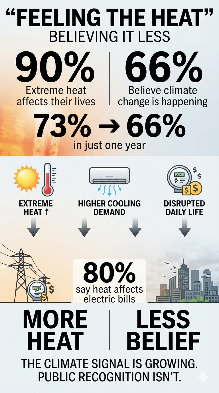
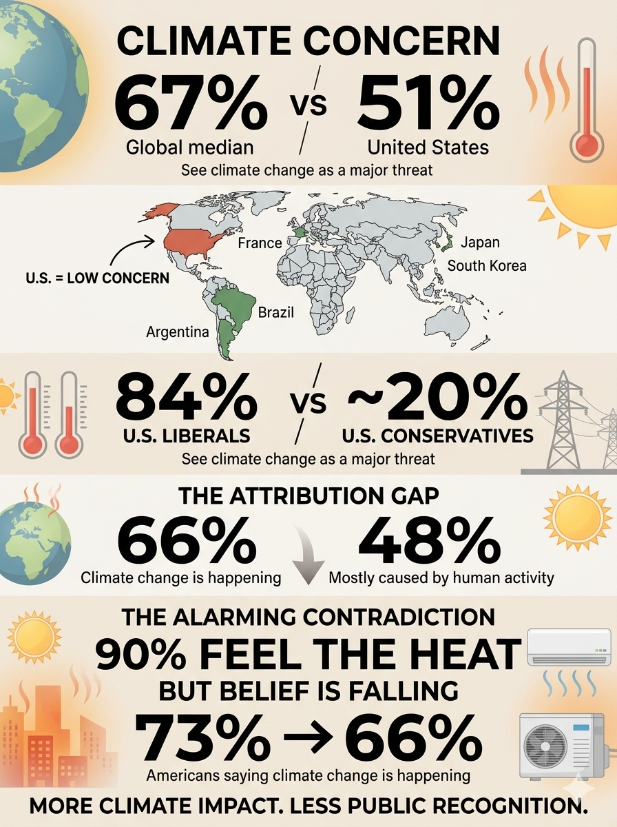
According to the poll, just 66% of Americans say climate change is happening, down sharply from 73% a year ago. That seven-percentage-point decline is particularly alarming because it comes at a time when Americans are reporting increasingly direct and disruptive experiences with extreme heat.

The disconnect raises an important question: How can people increasingly experience the consequences of a changing climate while becoming less likely to recognize climate change as the cause?

Extreme Heat Is Becoming Personal

The same poll found that 90% of Americans say extreme heat has affected their lives in some way, up from 83% in July 2024.

The impacts aren’t confined to abstract concerns about the environment. Americans report that extreme heat is affecting everyday life, including:

Electricity bills
Outdoor activities
Sleep
Travel and vacations
Daily routines

Perhaps most significantly, about 80% say extreme heat has affected their electricity bills, up from 69% in 2024.

In the Midwest, the increase is even more striking: 44% now say extreme heat has had a major impact on their electricity bills, compared with 29% two years ago.

That is climate change translated into something tangible: a higher household expense.

The Perception–Attribution Gap

The most important finding may not be the increase in heat-related disruption. It may be the growing gap between what Americans experience and what they believe is causing it.

The survey presents two seemingly contradictory trends:

90% say extreme heat has affected their lives.

Yet only 66% say climate change is happening.

And that 66% figure is down from 73% just one year ago.

This is a remarkable perception–attribution gap.

Americans can recognize that summers are becoming more difficult, electricity costs are rising, outdoor activities are being disrupted and extreme heat is affecting sleep—without necessarily connecting those experiences to a changing climate.

The result is a potentially dangerous disconnect between physical reality and public understanding.

Political Division Is Part of the Explanation

Political ideology continues to play an enormous role in how Americans interpret climate-related experiences.

Democrats are substantially more likely than Republicans to describe extreme heat as having a major impact on their lives. But that doesn’t mean Republicans aren’t experiencing the same heat.

The distinction is increasingly about interpretation and attribution.

People across the political spectrum can experience the same 100-degree day. They can experience the same oppressive humidity, pay the same higher electricity bill and face the same restrictions on outdoor activity.

But they may reach very different conclusions about why it is happening.

That distinction matters because climate change doesn’t require public agreement in order to produce physical consequences.

Climate Change Is Becoming an Economic Issue

The AP-NORC findings also demonstrate why climate change should not be viewed exclusively as an environmental issue.

Extreme heat creates a chain of consequences:

Higher temperatures → greater air-conditioning demand → higher electricity consumption → increased household costs

But that is only one pathway.

Extreme heat can also affect worker productivity, agriculture, infrastructure, public health, insurance losses and energy-grid reliability.

The household electricity bill may therefore be only the first visible economic manifestation of a much larger systemic problem.

The public doesn’t need to understand atmospheric physics to experience these consequences.

They simply need to notice that something is different.

The Most Alarming Finding Isn’t the Heat

The increase in extreme-heat impacts is concerning, but the seven-point decline in belief that climate change is happening may be even more alarming.

The country is experiencing a growing number of climate-related disruptions while simultaneously becoming less certain—or less willing—to identify climate change as the underlying cause.

That creates a dangerous situation for public policy.

Democratic societies depend upon the public recognizing problems before governments can effectively address them. If the physical impacts become increasingly severe while public recognition of their underlying causes declines, political pressure for adaptation and mitigation can weaken precisely when the need for action is growing.

This creates a potential feedback loop:

More climate disruption → greater personal impacts → greater economic costs → political polarization → weaker recognition of climate change → less public support for climate action → greater future vulnerability

That is not merely a communications problem.

It is a systemic risk.

Experience Is Increasing Faster Than Understanding

The AP-NORC poll doesn’t measure the physical climate system. It measures what Americans are experiencing and what they believe.

Those are different things.

The survey cannot establish how much of an individual’s electricity bill, sleep disruption or outdoor inconvenience is attributable specifically to climate change. Establishing those causal relationships requires observational climate data and scientific attribution studies.

But the poll does reveal something extremely important about the human response to climate change.

The consequences are becoming increasingly personal while public recognition of climate change is moving in the opposite direction.

That should concern everyone, regardless of political affiliation.

The challenge is no longer simply convincing people that the climate is changing.

It is explaining why their increasingly familiar experiences—extreme heat, higher cooling demand, disrupted outdoor activities, poor sleep and growing economic costs—are connected to a much larger physical system.

Americans may not agree about climate change.

But increasingly, they are living with its consequences.

And the most alarming finding from this poll is that as those consequences become harder to escape, fewer Americans say climate change is actually happening: 66% today, compared with 73% a year ago.

America Is an International Outlier on Climate Change

The decline in American belief becomes even more concerning when viewed against the rest of the world.

A 2025 Pew Research Center international survey of 25 countries found that a global median of 67% of respondents considered climate change a major threat to their country. In the United States, however, only 51% said the same—a gap of 16 percentage points.

The U.S. was among the least concerned countries surveyed. Americans were less likely than respondents in 13 of the 16 high-income countries included in the survey to view climate change as a major threat. In countries such as Argentina, Brazil, France, Japan and South Korea, roughly 80% of respondents regarded climate change as a major threat.

The difference is particularly striking because the United States is not insulated from climate impacts. Americans are experiencing extreme heat, rising cooling demand, disrupted outdoor activities and other consequences of a warming climate, yet concern about climate change remains comparatively low.

The American Divide Is Also Unusually Political

The international comparison becomes even more revealing when political ideology is considered.

Pew found that approximately 84% of U.S. liberals regarded climate change as a major threat, compared with only about 20% of U.S. conservatives. That enormous gap makes the United States an international outlier in the degree to which climate change has become politically polarized.

The result is a remarkable paradox.

Americans across the political spectrum can experience the same heat wave, pay the same electricity bill and endure the same disruption to their daily lives. Yet they may reach dramatically different conclusions about what those experiences mean.

The disagreement therefore isn’t simply about the physical environment. It is increasingly about how Americans interpret the physical environment.

Believing the Climate Is Changing Is Not the Same as Accepting Why

Another Pew measure illustrates the problem even more clearly.

In 2026, only 48% of Americans said the Earth is warming mostly because of human activity. That is substantially lower than the 66% who currently say climate change is happening in the AP-NORC poll.

The difference is crucial.

A person can acknowledge that the climate is changing without accepting that human activity is primarily responsible for that change. Others may accept human-caused warming but disagree about its severity, consequences or appropriate policy response.

This creates several layers of public perception:

Is the climate changing?

↓

Is human activity causing it?

↓

Is it becoming dangerous?

↓

Should government and society act?

Americans can answer those questions very differently.

An Alarming Combination

Taken together, the international and domestic polling reveals a troubling pattern:

90% — say extreme heat has affected their lives

80% — say heat has affected their electricity bills

73% → 66% — Americans saying climate change is happening

51% — Americans calling climate change a major national threat

48% — Americans saying warming is mostly caused by human activity

The numbers measure different things and should not be treated as interchangeable. But together they reveal a striking disconnect between experience, attribution and concern.

The United States is already an international outlier in climate skepticism and political polarization. Now, at a time when Americans report increasingly personal impacts from extreme heat, the share saying climate change is happening has fallen seven percentage points in only one year.

That may be the most troubling finding of all.

The physical climate signal is becoming harder to escape, while public recognition of that signal is moving in the opposite direction.

Strategic Petroleum Reserve Falls to Lowest Level Since 1983

Posted on 2026/08/06 by admin

As of July 31, 2026, the U.S. Strategic Petroleum Reserve (SPR) held approximately 304.8 million barrels of crude oil, its lowest level since March 1983.

From its historic peak of roughly 726 million barrels in 2009, the SPR has experienced a cumulative drawdown of approximately 421 million barrels—about a 58% reduction. The decline has been driven primarily by major emergency releases following Russia’s 2022 invasion of Ukraine and subsequent supply disruptions associated with instability in the Middle East in 2026.

The U.S. Energy Information Administration (EIA) estimates that the reserve could eventually fall to approximately 243 million barrels as currently authorized emergency release schedules conclude.

Strategic Risk: Erosion of U.S. Energy Security

The primary risk of reducing the SPR to approximately 243 million barrels is a severe loss of national energy security and geopolitical leverage during a major global crisis.

At that level—near the lowest inventory in more than four decades—the United States would have substantially less capacity to respond to an extended disruption in global oil supplies. A depleted reserve could also reduce the credibility and effectiveness of the SPR as a deterrent against supply shocks, geopolitical coercion, or major disruptions to global petroleum markets.

Structural and Infrastructure Risks

Cavern Structural Integrity

The SPR is stored in underground salt caverns that require careful management of pressure, oil levels, and cavern conditions. Repeatedly moving crude oil and fresh water into and out of these caverns can alter the physical characteristics of the salt formations and potentially increase operational and structural risks.

Maintaining the integrity of the caverns becomes increasingly important as the reserve is drawn down because the SPR’s ability to rapidly refill or sustain emergency withdrawals depends on the continued reliability of this underground storage infrastructure.

International Energy Agency Compliance

A substantially reduced SPR could also complicate U.S. compliance with International Energy Agency (IEA) emergency-stockholding requirements.

IEA member countries are generally required to maintain emergency oil stocks equivalent to at least 90 days of net oil imports. The relevant measure, however, is based on a country’s total qualifying emergency stocks—not simply the number of barrels held in the SPR. Therefore, the U.S. position must be evaluated using the full national stockholding calculation, including other qualifying inventories.

The Strategic Concern

The SPR was designed as a national insurance policy against severe and prolonged disruptions in petroleum supplies. Reducing the reserve by more than half from its 2009 peak fundamentally changes the country’s ability to absorb a major energy shock.

If inventories approach 243 million barrels, the United States would enter a period in which rebuilding the reserve could become increasingly important but potentially difficult. Large-scale purchases to replenish the SPR would require substantial funding, available crude supplies, suitable market conditions, and sufficient time.

The central strategic issue is therefore not simply how many barrels remain, but whether the United States retains enough readily deployable petroleum reserves to withstand a prolonged global supply disruption while simultaneously preserving the infrastructure, flexibility, and geopolitical leverage needed to respond to the next crisis.

Climate Change Today

Posted on 2026/07/282026/07/28 by admin

When Weather Becomes Climate

By Daniel Brouse

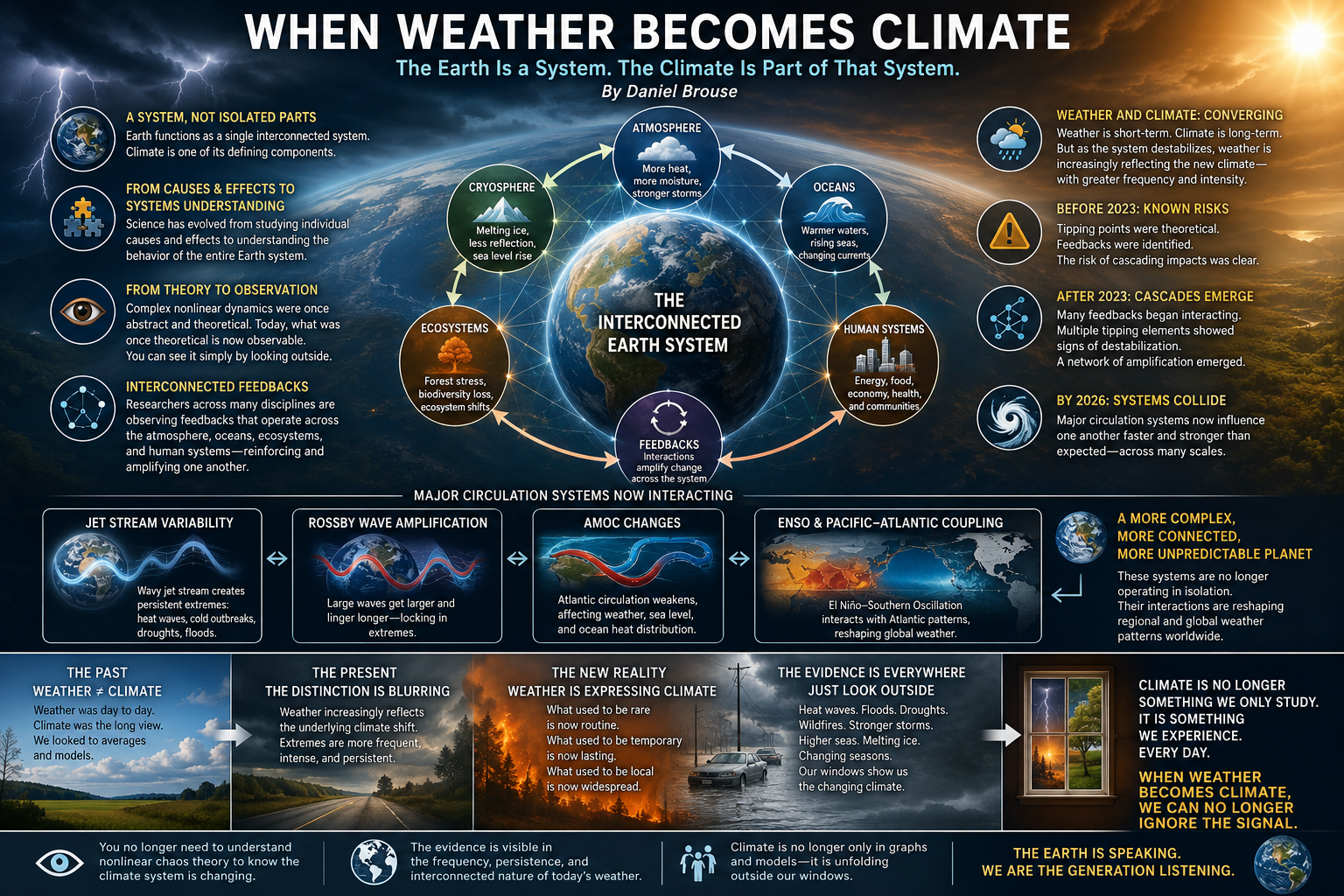
Earth functions as a single interconnected system, and climate is one of its defining components. For much of modern science, climatology focused primarily on identifying individual causes and effects. Today, that focus has expanded toward understanding the behavior of the entire Earth system.

The dynamics of complex nonlinear systems were once considered highly abstract, requiring sophisticated mathematical models to visualize their behavior. That is no longer the case. What was once theoretical has become increasingly observable. In many respects, the behavior of the climate system can now be seen simply by looking outside.

Climatologists, economists, ecologists, and other researchers are increasingly observing climate feedbacks operating across the entire Earth system. Rather than isolated events or independent variables, we are witnessing interconnected processes that reinforce one another across atmospheric, oceanic, ecological, and human systems.

Historically, weather and climate were treated as distinct concepts. Weather described short-term atmospheric conditions, while climate represented long-term statistical patterns. As the climate system becomes increasingly unstable, however, weather is reflecting those long-term changes with growing frequency and intensity. The distinction remains scientifically valid, but climate change is becoming visible through the character of everyday weather.

Before 2023, scientists understood that climate tipping points were possible, and numerous positive feedback mechanisms had already been identified. After 2023, evidence increasingly suggested that many of these feedbacks were interacting simultaneously, with multiple tipping elements showing signs of destabilization. Instead of isolated feedback loops, researchers began observing a network of interconnected processes capable of amplifying one another.

By 2026, many of Earth’s major circulation systems appear to be influencing one another in ways that are faster, stronger, and more interconnected than previously anticipated. These interactions are occurring across multiple scales, increasing the complexity of the global climate response.

Examples include the interaction between jet stream variability, Rossby wave amplification, and changes in the Atlantic Meridional Overturning Circulation (AMOC). Likewise, large-scale ocean-atmosphere interactions involving ENSO and Pacific–Atlantic climate coupling continue to reshape regional weather patterns around the globe.

Understanding the mathematics of nonlinear dynamics and chaos theory remains valuable, but it is no longer necessary to appreciate that the climate system is behaving differently. The evidence is increasingly visible in the frequency, persistence, and interconnected nature of the weather people experience.

In that sense, one of the defining characteristics of our time is that climate is no longer perceived only through long-term averages and scientific graphs. It is increasingly recognized through the weather unfolding outside our windows.

Why Weather Is Becoming Climate

The distinction between weather and climate has not disappeared. Weather remains the day-to-day state of the atmosphere, while climate describes long-term averages and the underlying behavior of the Earth system. What has changed is the degree to which climate is now shaping weather in real time.

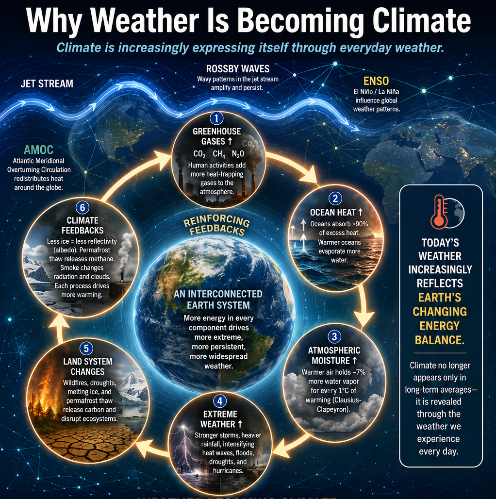
As greenhouse gases accumulate and the planet stores more heat, every component of the climate system contains more energy. Warmer oceans evaporate more water, the atmosphere holds more moisture, and circulation patterns are increasingly disrupted by changes in temperature gradients between the tropics and the poles. These changes alter not only the intensity of individual weather events but also the persistence and interaction of entire weather patterns.

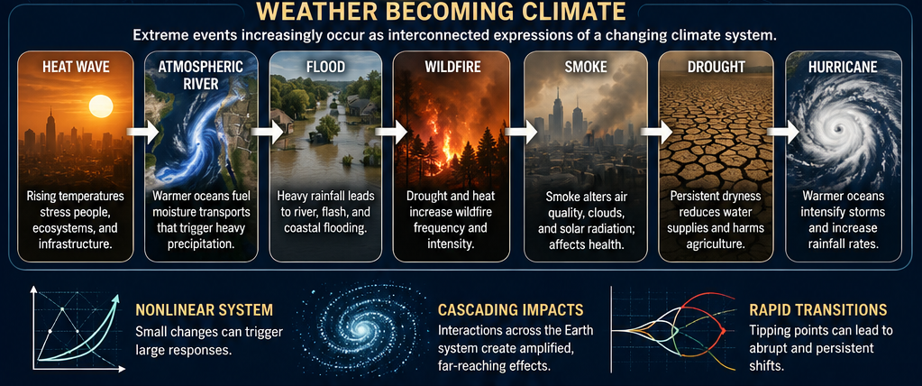
The result is a network of reinforcing feedbacks. A warming ocean fuels stronger atmospheric rivers and hurricanes. Droughts increase wildfire activity, while wildfire smoke alters atmospheric chemistry and solar radiation. Reduced snow and ice decrease Earth’s reflectivity, allowing additional warming. Permafrost thaw releases greenhouse gases that contribute to further warming. Each process influences others, producing cascading effects across the Earth system.

These interactions also affect the planet’s major circulation systems. Changes in the jet stream, Rossby wave amplification, ENSO, the Atlantic Meridional Overturning Circulation (AMOC), and other large-scale patterns increasingly influence one another. Rather than operating as largely independent phenomena, they are becoming components of an interconnected global system whose behavior is nonlinear and capable of rapid transitions.

This systems perspective helps explain why extreme weather events are becoming more persistent, widespread, and synchronized. Heat waves, floods, droughts, wildfires, and severe storms are no longer viewed simply as isolated disasters. They are increasingly understood as different expressions of the same underlying climate dynamics.

In this sense, weather has become one of the most visible indicators of climate change. The climate system is no longer revealing itself only through decades of averaged temperature records or scientific models. It is increasingly expressing itself through the weather that people experience every day. As nonlinear feedbacks continue to strengthen, weather is becoming the language through which climate communicates its changing state and at what rate.

What Fascinates You?

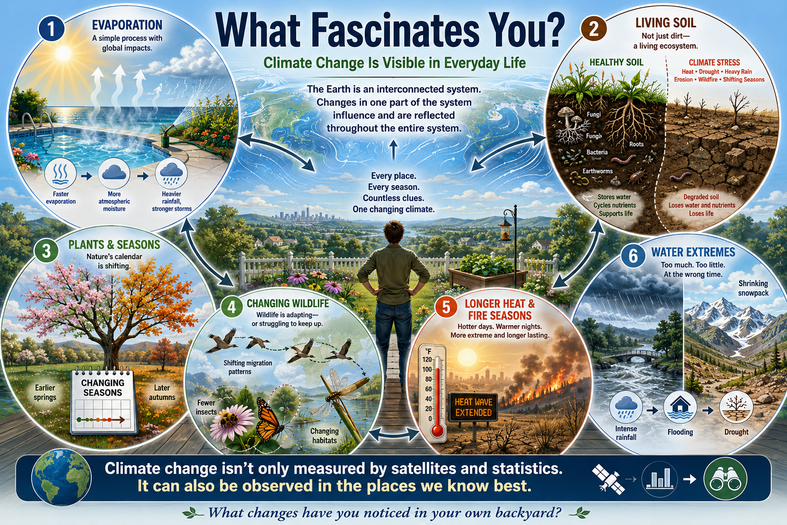
One of the remarkable aspects of climate change is that it no longer exists only in scientific journals or satellite imagery. It can be observed in countless ways during everyday life. Once you begin looking at the Earth as an interconnected system, signs of change seem to appear everywhere.

I find evaporation especially fascinating. It is one of the simplest processes to observe, yet it connects directly to the global climate system. I notice how quickly water disappears from a swimming pool after a hot, humid day. I see gardens requiring more frequent watering. At the global scale, the same process is evident in warmer oceans that transfer more water vapor into the atmosphere, fueling heavier downpours, stronger storms, and atmospheric rivers that are becoming increasingly familiar in regions where they were once uncommon.

I am equally fascinated by soil. Healthy soil is not simply dirt—it is a living ecosystem filled with fungi, bacteria, earthworms, insects, roots, and organic matter. It stores water, cycles nutrients, and supports nearly all terrestrial life. Yet I also see soil under stress. Extended heat, drought, intense rainfall, erosion, wildfire, and changing seasons are degrading soils in many places. The ground beneath our feet is quietly telling the story of a changing climate.

Others may notice different changes. Some watch the timing of blossoms in the spring or leaves in the autumn. Others observe declining insect populations, shifting bird migrations, warmer nights, disappearing snow cover, longer wildfire seasons, or increasingly persistent heat waves. Farmers may recognize changing growing seasons, while anglers notice warmer streams and changing fish populations. Every landscape offers its own clues.

Climate change is often discussed in terms of global averages and long-term statistics, but it is also a collection of countless local observations. The Earth system expresses itself through the places we know best.

So, what fascinates you?

What changes have you noticed in your own backyard, neighborhood, or community? The answers to that question may be among the most compelling evidence that weather is increasingly revealing the changing character of our climate.

Climate Change and a Backyard Produce Experiment

Posted on 2026/07/27 by admin

by Daniel Brouse

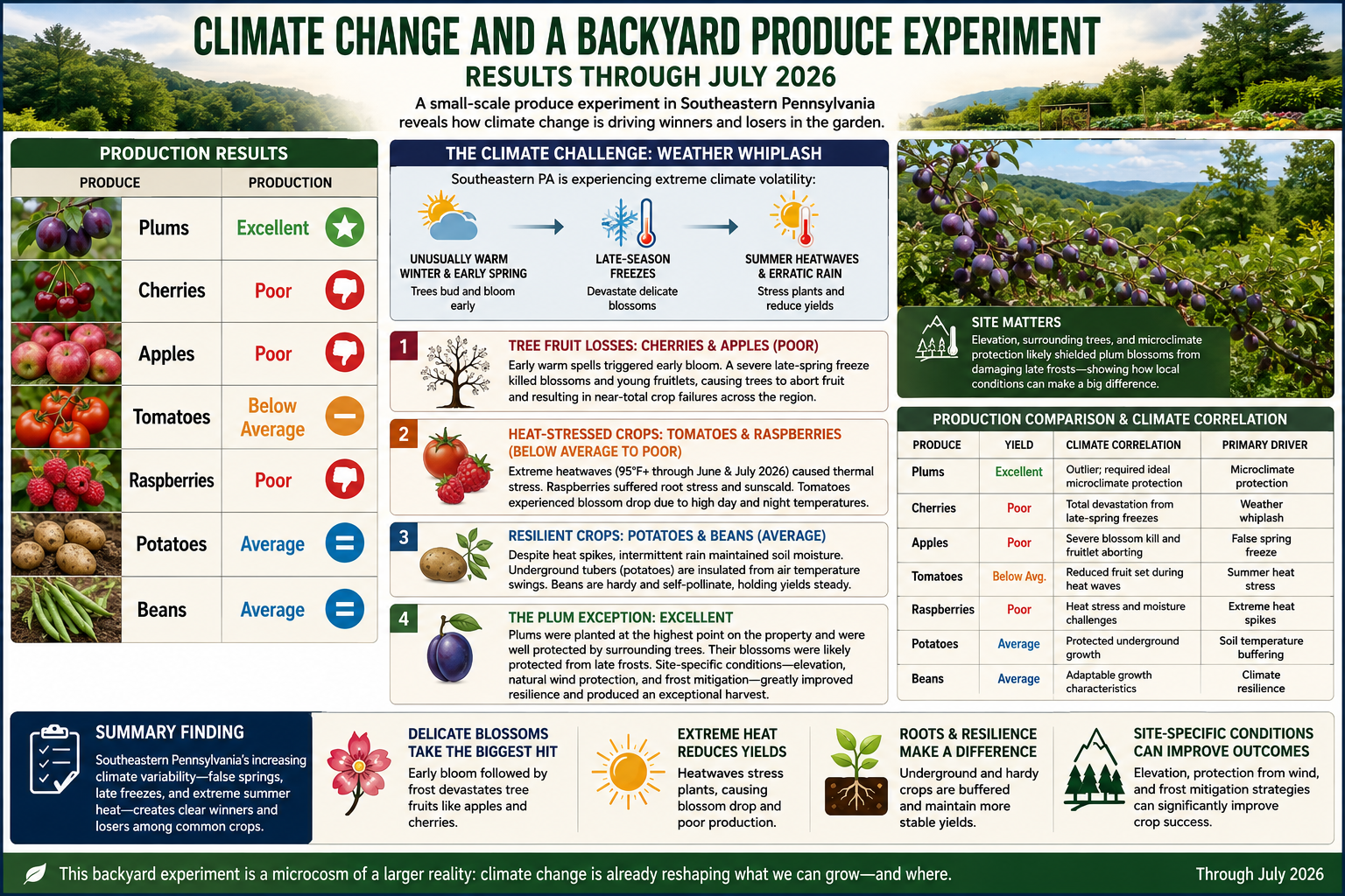
Climate Change and a Backyard Produce Experiment: Results Through July 2026

Production Results

Produce	Production
Plums	Excellent
Cherries	Poor
Apples	Poor
Tomatoes	Below Average
Raspberries	Poor
Potatoes	Average
Beans	Average

Introduction

The results of this backyard produce experiment closely reflect the climate-related agricultural challenges affecting Southeastern Pennsylvania through July 2026. The region has experienced increasing climate volatility, often described as “weather whiplash”—a pattern characterized by unusually warm winter and early spring conditions followed by damaging late-season freezes, summer heat waves, and increasingly erratic precipitation.

The observed performance of each crop corresponds closely with the climatic stresses documented throughout the region.

Analysis by Crop Type

1. Tree Fruit Losses: Cherries and Apples

Both cherries and apples produced poor yields, mirroring the severe losses reported by many Pennsylvania fruit growers.

Climate Driver:
Warmer winters and early springs are causing fruit trees to break dormancy and bloom earlier than historical averages.

The False Spring Effect:
Following an unusually warm early spring, a significant late-season freeze struck Pennsylvania. Because many cherry and apple trees had already reached vulnerable flowering stages, blossoms were damaged or destroyed. Trees subsequently aborted damaged fruitlets, resulting in dramatically reduced harvests.

Observed Result: Poor production.

2. Heat-Stressed Crops: Tomatoes and Raspberries

Tomatoes and raspberries showed substantial sensitivity to elevated summer temperatures.

Climate Driver:
Repeated heat waves during June and July 2026 produced prolonged periods with temperatures exceeding 95°F (35°C).

Botanical Impacts:

Raspberries possess shallow root systems that are highly vulnerable to heat stress and soil moisture fluctuations. Prolonged high temperatures can reduce berry size, quality, and overall production.
Tomatoes often experience blossom drop when both daytime and nighttime temperatures remain elevated. Flowers fail to pollinate successfully, reducing fruit set and overall yield.

Observed Results:

Raspberries: Poor
Tomatoes: Below Average

3. Resilient Crops: Potatoes and Beans

Potatoes and beans demonstrated greater resilience despite challenging weather conditions.

Climate Driver:
Although extreme heat occurred, the season also included intermittent rainfall events that helped maintain soil moisture.

Botanical Impacts:

Potatoes benefit from underground tubers that remain insulated from extreme air temperatures.
Beans are generally adaptable and capable of maintaining stable production across a wider range of environmental conditions.

Observed Results:

Potatoes: Average
Beans: Average

4. The Plum Exception

Plums were the clear standout of the experiment, producing an excellent harvest despite widespread challenges affecting other fruit crops.

Climate Driver:
Most stone fruit in the region faced significant frost damage. However, localized factors can substantially alter outcomes.

Possible Explanations:

Favorable microclimate conditions
Higher-elevation planting sites where cold air drains away
Natural frost protection from surrounding terrain
Orchard management practices that reduced freeze damage

The plums were planted at the highest point on the property and were well protected by surrounding trees. Their elevated location likely reduced frost exposure, while the surrounding trees helped moderate temperature fluctuations and wind. Together, these conditions likely protected the blossoms from the damaging late-spring frosts that devastated many other fruit trees. The exceptional performance of the plum crop suggests that site-specific conditions—including elevation, natural wind protection, and frost mitigation—can significantly improve a crop’s resilience to climate-related stresses.

Observed Result: Excellent production.

Production Comparison and Climate Correlation

Produce	Yield	Climate Correlation	Primary Driver
Plums	Excellent	Localized success despite regional stress	Microclimate protection
Cherries	Poor	Severe blossom losses from spring freeze	Weather whiplash
Apples	Poor	Frost-damaged blossoms and fruitlets	False spring freeze
Tomatoes	Below Average	Reduced fruit set during heat waves	Summer heat stress
Raspberries	Poor	Heat stress and moisture challenges	Extreme temperatures
Potatoes	Average	Protected underground growth	Soil temperature buffering
Beans	Average	Adaptable growth characteristics	Climate resilience

Conclusions

This small-scale produce experiment provides a useful illustration of how climate change is increasingly influencing agricultural outcomes in Southeastern Pennsylvania.

The results reflect a broader regional pattern:

Early warming followed by hard freezes disproportionately impacts tree fruits such as apples and cherries.
Extreme summer heat reduces yields of temperature-sensitive crops such as tomatoes and raspberries.
Root crops and legumes generally demonstrate greater resilience to short-term temperature extremes.
Microclimate advantages can sometimes offset regional climate pressures, as demonstrated by the exceptional plum harvest.

Key Finding

The experiment suggests that Southeastern Pennsylvania’s increasing climate variability—particularly the combination of false springs, late freezes, and extreme summer heat—is creating clear winners and losers among common food crops. Delicate flowering fruit trees experienced the greatest losses, while more resilient crops maintained average production levels despite challenging conditions.

The Two Sides of the Climate Crisis: Consumption and Production

Posted on 2026/07/25 by admin

by Daniel Brouse

Climate change is often discussed as a problem of emissions, but emissions are the result of two interconnected forces: consumption and production.

Q: What are the greatest drivers of climate change?
A: Consumption and production.

At present, I would rank our addiction to consumption and ecofascism as the two most significant drivers of the climate crisis. While they operate in different ways, both reinforce the systems that accelerate environmental degradation.

The Consumption Problem

The United States, Western Europe, Canada, and Australia represent some of the world’s most consumption-driven economies. When self-interest, materialism, and short-term economic incentives dominate decision-making, consumer demand becomes one of the primary drivers of climate change, influencing not only greenhouse gas emissions but also land-use change, deforestation, habitat destruction, water consumption, resource depletion, and biodiversity loss.

This is why consumption-based accounting provides a more accurate picture of climate responsibility than production-based accounting alone.

For example, if a smartphone is manufactured in Asia using coal-generated electricity and then shipped across the Pacific to a consumer in Los Angeles, the emissions from mining, manufacturing, transportation, and delivery are ultimately driven by the purchasing decision. Under consumption-based accounting, those emissions are attributed to the American consumer rather than solely to the country where the phone was manufactured.

Read the full explanation and view the rankings here:

http://membrane.com/global_warming/Accounting-for-Climate-Responsibility.html#the-carbon-we-own

The Production Problem

The production side of the equation is likewise influenced by self-interest and economic incentives, but it is also shaped by ideological movements that obstruct effective climate action.

Two distinct, though sometimes overlapping, ideologies are particularly important:

Denialism is characterized by the rejection of scientific evidence, refusal to engage with empirical data, and reliance on misinformation or rhetorical distraction. Its primary objective is often the protection of political, ideological, or economic interests by undermining the scientific consensus.

Ecofascism combines elements of denialism with authoritarian, exclusionary, or extremist beliefs. In its most extreme forms, it portrays environmental collapse as acceptable—or even desirable—because it is viewed as reducing populations or preserving resources for groups considered more deserving than others. This ideology has historically been associated with racist, xenophobic, or eugenicist beliefs and rejects principles of equality and shared human responsibility.

The distinction is important. Traditional denialism primarily seeks to delay or prevent climate policy. Ecofascism goes further by framing unequal human survival as an acceptable or even desirable outcome — eliminationist logic.

Why This Matters

Climate change is not simply a technological or economic challenge. It is also a question of values.

On one side, excessive consumption drives demand for fossil fuels, resource extraction, and emissions. On the other, ideologies that reject science or rationalize unequal human suffering weaken society’s ability to respond effectively to the crisis.

Both sides must be addressed if meaningful progress is to be made.

The States with the Biggest Climate Footprints Aren’t the Ones You Think

Posted on 2026/07/24 by admin

by Daniel Brouse

When most people think about greenhouse gas emissions, they picture sprawling cities, crowded highways, and millions of people flipping on lights and air conditioners. It’s no surprise, then, that states like California, Texas, Florida, and New York usually dominate lists of greenhouse gas emissions. But those rankings tell only part of the story.

What if the question isn’t simply “Which states emit the most greenhouse gases?” What if it’s “Which states are most responsible for producing the fossil fuels that drive climate change?”

The answer looks dramatically different.

Beyond Smokestacks and Tailpipes

Traditional greenhouse gas inventories are based on territorial emissions—the emissions that physically occur within a state’s borders. That includes electricity generation, transportation, manufacturing, agriculture, and buildings.

This accounting system is useful, but it overlooks much of the climate impact associated with fossil fuel production.

Before a gallon of gasoline reaches your car or natural gas heats your home, fossil fuels must be:

explored,
extracted,
processed,
transported,
refined,
and stored.

Each of these steps releases greenhouse gases. Oil wells leak methane. Coal mines vent methane. Natural gas fields flare excess gas. Refineries consume enormous amounts of energy. LNG export terminals require massive refrigeration systems. Petrochemical plants emit carbon dioxide while transforming hydrocarbons into fuels and plastics.

These emissions are real. Yet many are only partially reflected—or entirely absent—from conventional state comparisons.

Introducing the Composite Climate Responsibility Index

To capture the full climate burden of fossil fuel production, I developed the Composite Climate Responsibility Index (CCRI).

Rather than looking only at emissions released within a state’s borders, CCRI combines four major components:

Territorial emissions – direct greenhouse gas emissions occurring within the state.
Upstream emissions – methane leakage, venting, flaring, and other fugitive releases.
Processing emissions – petroleum refining, LNG facilities, natural gas processing, and petrochemical manufacturing.
Extraction emissions – emissions associated with coal mining, oil production, drilling, hydraulic fracturing, and natural gas extraction.

The combined total is then divided by the state’s population to produce a per-capita measure of climate responsibility.

This approach shifts the focus from where emissions occur to where the fossil fuel system originates.

A Completely Different Ranking

Applying this framework produces a ranking that bears little resemblance to traditional greenhouse gas inventories.

Instead of being dominated by the largest population centers, the states with the highest per-capita climate responsibility are overwhelmingly those that produce fossil fuels.

Top Ten States by Composite Climate Responsibility

Wyoming
North Dakota
West Virginia
New Mexico
Louisiana
Alaska
Oklahoma
Texas
Pennsylvania
Kentucky

Notice who’s missing.

California, Florida, New York, New Jersey, Massachusetts, and Washington—all states commonly associated with high emissions because of their large populations—drop dramatically in the rankings.

Instead, relatively small states become climate heavyweights because they extract, refine, process, or export enormous quantities of fossil fuels.

Wyoming: A Climate Giant with Half a Million People

Wyoming is home to fewer than 600,000 residents, yet it produces more coal than any other state and remains a major producer of natural gas.

Under conventional accounting, Wyoming appears to have modest total emissions simply because so few people live there.

But when coal mining, methane releases, and extraction activities are included, Wyoming’s per-capita climate burden becomes extraordinary.

Its climate footprint is measured not by how many people live there, but by how much carbon leaves the state embedded in coal, oil, and natural gas.

Texas: The Carbon Superpower

Texas remains in a category of its own.

No other state combines:

the nation’s largest oil production,
the largest natural gas production,
the largest refining capacity,
one of the world’s largest petrochemical industries,
extensive LNG export facilities,
and the highest total greenhouse gas emissions.

Its enormous population moderates its per-capita ranking, but Texas still lands in the top ten because the scale of its fossil fuel industry is unmatched.

In absolute terms, Texas likely contributes more lifecycle greenhouse gas emissions than any other U.S. state.

Methane Changes Everything

One of the largest differences between CCRI and conventional inventories is methane.

Natural gas has often been marketed as a “cleaner” fossil fuel because it emits less carbon dioxide when burned than coal.

However, methane itself is a potent greenhouse gas. Even relatively small leaks during drilling, gathering, processing, and transportation can substantially increase the climate impact of natural gas production.

States with large oil and gas industries—such as New Mexico, North Dakota, Pennsylvania, Oklahoma, and Louisiana—move sharply upward once methane leakage, venting, and flaring are included.

Ignoring upstream methane is like calculating the cost of owning a car while pretending gasoline is free.

Production Matters

The key insight of CCRI is that climate responsibility does not end where emissions occur.

A barrel of oil extracted in North Dakota may be refined in Louisiana, transported through Texas, shipped overseas, and ultimately burned in Europe or Asia.

Each step adds greenhouse gases.

Traditional inventories divide these emissions among multiple jurisdictions, often obscuring the role of the states that initiated the fossil fuel supply chain.

CCRI reconnects those pieces.

It recognizes that extraction, processing, and upstream emissions are not incidental—they are essential components of fossil fuel production.

A More Complete Picture

The Composite Climate Responsibility Index is not intended to replace traditional greenhouse gas inventories. Those inventories remain indispensable for tracking progress toward emissions reduction within individual states.

Instead, CCRI complements existing accounting by expanding the system boundary to include the activities that make fossil fuel consumption possible.

This broader perspective helps answer questions that territorial inventories cannot:

Which states produce the largest share of climate-forcing emissions?
Where would methane reductions have the greatest impact?
Which regions contribute disproportionately to fossil fuel supply?
How should climate responsibility be allocated in a production-based economy?

By incorporating extraction, processing, upstream methane, and direct emissions into a single per-capita metric, CCRI reveals a reality that traditional rankings often miss: the states producing the fuels that power the global economy are frequently those carrying the largest climate responsibility—even when their populations are relatively small.

In the coming years, as policymakers increasingly focus on lifecycle emissions, methane mitigation, and supply-side climate policy, production-based metrics such as CCRI may prove to be as important as the territorial inventories that have guided climate reporting for decades.

Global Comparison

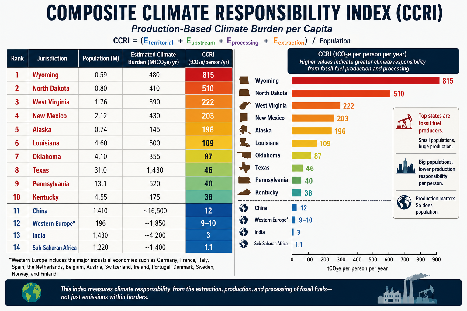
A comparison becomes especially revealing when the same production-based accounting is applied to both U.S. states and world regions. Instead of asking who burns the carbon, the CCRI asks who produces and enables the fossil carbon economy.

The formula remains: $CCRI=\frac{E_{territorial}+E_{upstream}+E_{processing}+E_{extraction}}{P}$ CCRI=PEterritorial+Eupstream+Eprocessing+Eextraction

Using this methodology, the comparison changes dramatically from conventional per-capita emissions rankings.

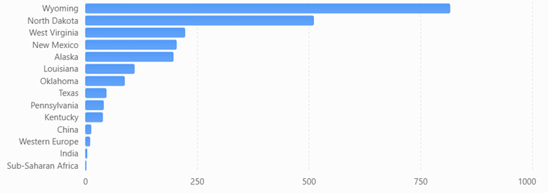
Estimated Composite Climate Responsibility

Rank	Jurisdiction	Population (M)	Estimated Climate Burden (MtCO₂e/yr)	CCRI (tCO₂e/person/yr)
1	Wyoming	0.59	480	815
2	North Dakota	0.80	410	510
3	West Virginia	1.76	390	222
4	New Mexico	2.12	430	203
5	Alaska	0.74	145	196
6	Louisiana	4.60	500	109
7	Oklahoma	4.10	355	87
8	Texas	31.0	1,430	46
9	Pennsylvania	13.1	520	40
10	Kentucky	4.55	175	38
11	China	1,410	~16,500	≈12
12	Western Europe*	196	~1,850	≈9–10
13	India	1,430	~4,200	≈3
14	Sub-Saharan Africa	1,220	~1,400	≈1.1

*Western Europe includes the major industrial economies such as Germany, France, Italy, Spain, the Netherlands, Belgium, Austria, Switzerland, Ireland, Portugal, Denmark, Sweden, Norway, and Finland.

Composite Climate Responsibility Index (CCRI)

Estimated production-based climate burden per capita using territorial emissions, extraction, processing, and upstream emissions.

What the comparison shows

Several important conclusions emerge.

First, fossil fuel production is far more geographically concentrated than fossil fuel consumption. Wyoming’s estimated production-based climate burden is roughly 68 times higher per resident than China’s, despite China’s position as the world’s largest emitter under conventional territorial accounting. The difference reflects Wyoming’s role as a major coal and natural gas producer serving markets far beyond its borders.

Second, China’s ranking changes substantially under the CCRI framework. China remains a major contributor because of its large coal industry, extensive refining capacity, and industrial base, but its enormous population reduces its per-capita production burden to around 12 tCO₂e per person, well below several U.S. fossil-fuel-producing states.

Third, Western Europe falls even lower. While it retains significant refining and industrial capacity, domestic fossil fuel extraction has declined over several decades. Much of its energy is imported, so a production-based metric attributes a smaller share of upstream responsibility than a consumption-based metric would.

Fourth, India and Sub-Saharan Africa rank near the bottom. Although both regions have growing energy demand, their per-capita fossil fuel production and associated upstream emissions remain comparatively low. Their climate burden is driven primarily by domestic energy use rather than large-scale extraction and export industries.

A different perspective on climate responsibility

Traditional greenhouse gas inventories emphasize where emissions occur. The CCRI instead emphasizes where the fossil fuel supply chain begins. These are complementary perspectives, each useful for different policy questions.

Territorial inventories help governments manage emissions within their borders.
Consumption-based inventories assign responsibility to the end user of goods and energy.
The CCRI highlights the jurisdictions that extract, process, and prepare fossil fuels for global consumption.

Together, these three accounting systems provide a more complete understanding of climate responsibility. The comparison also illustrates that some of the world’s highest production-based climate burdens are found not in entire countries, but in a handful of resource-rich U.S. states whose fossil fuel industries serve national and international markets.

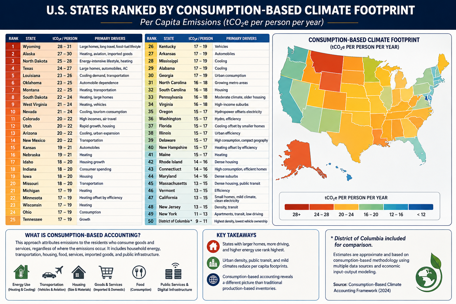
State Your Climate State

Posted on 2026/07/24 by admin

Estimated Consumption-Based Climate Footprint

(tCO₂e per person per year)

Rank	State	Estimated Footprint	Primary Drivers
1	Wyoming	28–31	Large homes, long travel distances, fossil-fuel lifestyle
2	Alaska	27–30	Heating, aviation, imported goods
3	North Dakota	25–28	Energy-intensive lifestyle, heating
4	Texas	24–27	Large homes, automobiles, air conditioning
5	Louisiana	23–26	Cooling demand, transportation
6	Oklahoma	23–25	Automobile dependence
7	Montana	22–25	Heating, transportation
8	South Dakota	22–24	Heating, large homes
9	West Virginia	21–24	Heating, vehicles
10	Nevada	21–24	Cooling, tourism consumption
11	Colorado	20–22	High incomes, air travel
12	Utah	20–22	Rapid growth, housing
13	Arizona	20–22	Cooling, urban expansion
14	New Mexico	20–22	Transportation
15	Kansas	19–21	Automobiles
16	Nebraska	19–21	Heating
17	Idaho	18–20	Housing growth
18	Indiana	18–20	Consumer spending
19	Iowa	18–20	Housing
20	Missouri	18–20	Transportation
21	Michigan	17–19	Heating
22	Minnesota	17–19	Heating offset by efficiency
23	Wisconsin	17–19	Heating
24	Ohio	17–19	Consumption
25	Tennessee	17–19	Growth
26	Kentucky	17–19	Vehicles
27	Arkansas	17–19	Automobiles
28	Mississippi	17–19	Cooling
29	Alabama	17–19	Cooling
30	Georgia	17–19	Urban consumption
31	North Carolina	16–18	Growing metro areas
32	South Carolina	16–18	Housing
33	Pennsylvania	16–18	Moderate climate, older housing
34	Virginia	16–18	High-income suburbs
35	Oregon	15–17	Hydropower offsets electricity
36	Washington	15–17	Hydro, efficiency
37	Florida	15–17	Cooling offset by small homes
38	Illinois	15–17	Urban efficiency
39	Delaware	15–17	High consumption, compact geography
40	New Hampshire	15–17	Heating offset by efficiency
41	Maine	15–17	Heating
42	Rhode Island	14–16	Dense housing
43	Connecticut	14–16	High consumption, efficient homes
44	Maryland	14–16	Dense suburbs
45	Massachusetts	13–15	Dense housing, public transit
46	Vermont	13–15	Efficiency
47	California	13–15	Small homes, mild climate, clean electricity
48	New Jersey	13–15	Density, transit
49	New York	11–13	Apartments, transit, low driving
50	District of Columbia*	9–11	Highest density, lowest vehicle ownership

(*Included for comparison.)

Accounting Method

Using the methodology from your consumption-based accounting paper, the rankings would look quite different from conventional state CO₂ inventories. Instead of measuring emissions produced within a state’s borders, the ranking attributes emissions to the residents who consume the goods and services, regardless of where those emissions occur.

The principal variables would include:

Household energy consumption
Heating and cooling demand
Transportation (vehicle ownership, VMT, aviation)
Housing size
Household income and purchasing power
Consumption of imported manufactured goods
Food consumption
Public and private services
Data center and digital infrastructure usage
Construction materials and embodied carbon

Because imported goods are attributed to consumers, states with high incomes and high levels of consumption generally rise in the rankings, while manufacturing states fall relative to production-based inventories.

What stands out?

Highest per-capita footprints

These states combine several characteristics:

Large single-family homes
Long commuting distances
High vehicle ownership
Significant heating or cooling demand
Frequent air travel
Higher embodied consumption in housing and infrastructure

Texas, Alaska, Wyoming, and North Dakota score highly not simply because of fossil-fuel production, but because residents tend to consume more energy per person.

Lowest per-capita footprints

The Northeast and California benefit from:

Smaller living spaces
Greater urban density
More public transportation
Lower vehicle miles traveled
Cleaner electricity
Higher building efficiency

New York illustrates the effect well. Although it has one of the largest economies in the world, the average resident lives in a much smaller dwelling, drives less, and relies more on mass transit than residents of most other states, resulting in one of the lowest per-capita consumption footprints.

Comparison with traditional accounting

Under conventional EPA production-based accounting:

Texas is by far the largest emitter because of industry and energy production.
California appears relatively high due to its large economy.
Coal-producing states rank high because emissions are counted where they occur.

Under consumption-based accounting, the question changes to:

“How much climate impact does the average resident’s lifestyle require?”

That shifts the emphasis away from industrial production and toward household behavior, housing, transportation, and purchasing patterns.

For an even more rigorous version suitable for publication, you could develop a state-level Multi-Regional Input-Output (MRIO) model analogous to your international consumption framework. Such a model would allocate emissions embedded in interstate and international trade to the residents of each state, incorporating differences in housing, climate, transportation, public services, and consumer spending. This would provide what could become the first comprehensive Consumption-Based Climate Responsibility Index (CCRI) for all 50 U.S. states.

US States Climate Change Rankings

Posted on 2026/07/24 by admin

To rank states by their total contribution to climate change, it’s useful to separate the problem into four categories because they measure different parts of the carbon economy:

Direct GHG emissions (what is emitted within the state)
Fossil fuel extraction (coal, oil, natural gas removed from the ground)
Fossil fuel production and processing (refining, LNG, petrochemicals, etc.)
Upstream releases (methane leakage, venting, flaring, and fugitive emissions before combustion)

Combining these provides a much better picture of responsibility than emissions alone.

Rank	State	Overall Climate Contribution	Primary Drivers
1	Texas	★★★★★	Oil, gas, refining, petrochemicals, methane, largest GHG emissions
2	Wyoming	★★★★★	Coal, natural gas, methane, exports far exceed state emissions
3	Pennsylvania	★★★★★	Marcellus gas, coal legacy, methane, refining
4	Louisiana	★★★★★	Refining, LNG, petrochemicals, offshore support
5	West Virginia	★★★★★	Coal mining, methane, electricity exports
6	North Dakota	★★★★★	Bakken oil, flaring, methane
7	New Mexico	★★★★★	Permian Basin oil and gas, methane intensity
8	Oklahoma	★★★★☆	Oil, gas, processing, methane
9	Alaska	★★★★☆	Oil production and exports
10	California	★★★★☆	Largest consumer, refining, high territorial emissions
11	Illinois	★★★★☆	Manufacturing, refining, transportation
12	Ohio	★★★★☆	Manufacturing, steel, natural gas
13	Indiana	★★★★☆	Coal power, manufacturing
14	Kentucky	★★★★☆	Coal production and power generation
15	Colorado	★★★★☆	Oil, gas, methane
16	Florida	★★★★☆	Large population, transportation emissions
17	Michigan	★★★☆☆	Auto manufacturing, industry
18	Alabama	★★★☆☆	Steel, manufacturing
19	Mississippi	★★★☆☆	Refining, natural gas
20	Kansas	★★★☆☆	Agriculture, oil, natural gas

By Direct GHG Emissions

Approximate order:

Texas
California
Pennsylvania
Florida
Louisiana
Illinois
Ohio
Indiana
Michigan
New York

By Fossil Fuel Extraction

Texas
Wyoming
Pennsylvania
New Mexico
North Dakota
West Virginia
Oklahoma
Colorado
Alaska
Kentucky

By Oil Production

Texas
New Mexico
North Dakota
Alaska
California
Colorado
Oklahoma
Louisiana
Wyoming
Utah

By Natural Gas Production

Texas
Pennsylvania
Louisiana
West Virginia
Oklahoma
New Mexico
Ohio
Colorado
Wyoming
Arkansas

By Coal Production

Wyoming
West Virginia
Pennsylvania
Illinois
Kentucky
Montana
North Dakota
Indiana
Colorado
Alabama

By Upstream Methane Releases

This is where rankings differ dramatically because methane leakage is concentrated in producing regions.

Texas
New Mexico
Pennsylvania
Louisiana
North Dakota
Wyoming
Oklahoma
Colorado
West Virginia
Alaska

By Refining & Petrochemicals

Texas
Louisiana
California
Illinois
Pennsylvania
Oklahoma
Indiana
Mississippi
New Jersey
Washington

Overall Climate Burden Index

If I were constructing a composite index weighted approximately as:

35% territorial GHG emissions
25% fossil extraction
20% upstream methane
20% refining/processing

the top ten would likely be:

Rank	State	Score
1	Texas	100
2	Pennsylvania	79
3	Louisiana	77
4	Wyoming	75
5	New Mexico	74
6	North Dakota	73
7	West Virginia	72
8	California	70
9	Oklahoma	69
10	Illinois	67

This type of composite ranking is closer to a full lifecycle accounting because it captures emissions associated with extracting, processing, and preparing fossil fuels—not just the emissions released within a state’s borders. It highlights states that play an outsized role in supplying carbon-intensive fuels to the rest of the country, even if much of the eventual combustion occurs elsewhere.

Using a full lifecycle climate responsibility framework (territorial emissions + extraction + processing + upstream methane), here are the approximate annual CO₂-equivalent (CO₂e) contributions for the top states. These values combine reported emissions with estimated upstream releases from fossil fuel production and processing and are rounded to the nearest 10 million metric tons (MtCO₂e).

Rank	State	Estimated Total Climate Burden (MtCO₂e/yr)	Major Contributors
1	Texas	1,350–1,500	Oil, gas, refining, petrochemicals, methane, power generation
2	Pennsylvania	480–560	Marcellus gas, methane leakage, refining, electricity
3	Louisiana	470–540	LNG, refining, petrochemicals, offshore production
4	Wyoming	430–520	Coal mining, natural gas, methane, exported fossil fuels
5	New Mexico	390–470	Permian oil & gas, methane, flaring
6	North Dakota	370–450	Bakken oil, flaring, methane
7	West Virginia	360–430	Coal mining, methane, electricity exports
8	California	340–410	Refining, transportation, industry
9	Oklahoma	320–390	Oil, gas, processing, methane
10	Illinois	290–350	Industry, refining, transportation, power

For comparison: territorial emissions alone

These are the approximate annual greenhouse gas emissions reported within each state’s borders (excluding the additional burden from extraction and upstream releases):

Rank	State	Territorial GHG (MtCO₂e/yr)
1	Texas	~760
2	California	~360
3	Pennsylvania	~250
4	Florida	~230
5	Louisiana	~220
6	Illinois	~210
7	Ohio	~200
8	Indiana	~195
9	Michigan	~180
10	New York	~170

Full lifecycle vs. territorial accounting

The difference between the two rankings highlights why a lifecycle approach matters:

Texas nearly doubles its climate footprint once upstream methane, refining, and extraction are included.
Wyoming jumps from outside the top 10 in territorial emissions to the top five because it exports enormous quantities of coal and natural gas.
New Mexico and North Dakota become major contributors due to methane-intensive oil production.
Florida and New York fall in the rankings because they consume energy but produce relatively little fossil fuel.
Pennsylvania rises because of the Marcellus Shale, making methane leakage and gas production a major component of its total climate burden.

Estimated Composite Per-Capita Climate Burden

Rank	State	Population (M)	Total Burden (MtCO₂e)	tCO₂e/person/yr
1	Wyoming	0.59	480	≈815
2	North Dakota	0.80	410	≈510
3	New Mexico	2.12	430	≈203
4	Louisiana	4.60	500	≈109
5	West Virginia	1.76	390	≈222
6	Alaska	0.74	145	≈196
7	Texas	31.0	1,430	≈46
8	Oklahoma	4.10	355	≈87
9	Pennsylvania	13.1	520	≈40
10	Kentucky	4.55	175	≈38

Next Tier

Rank	State	tCO₂e/person
11	Colorado	~34
12	Indiana	~31
13	Mississippi	~29
14	Illinois	~25
15	Ohio	~23
16	Alabama	~23
17	Montana	~22
18	California	~10
19	Florida	~10
20	New York	~9

Visualizing the disparity

The contrast is striking:

State	Composite Per Capita (tCO₂e/person)	Relative to U.S. Average (~22)
Wyoming	815	37×
North Dakota	510	23×
West Virginia	222	10×
New Mexico	203	9×
Alaska	196	9×
Louisiana	109	5×
Oklahoma	87	4×
Texas	46	2×
Pennsylvania	40	1.8×
California	10	0.45×
New York	9	0.4×

Interpretation

This metric reveals that many of the largest contributors are energy-exporting states rather than the most populous ones:

Wyoming dominates because a small population supports one of the world’s largest coal and fossil-fuel export industries.
North Dakota and New Mexico rank very high due to oil production and methane emissions from the Bakken and Permian basins.
Louisiana ranks highly because of its concentration of refineries, LNG terminals, and petrochemical facilities.
Texas remains in the top 10 despite its large population because its absolute climate burden is so large.
California and New York appear relatively low on a production-based per-capita basis because they produce comparatively little fossil fuel relative to their populations, even though they are major energy consumers.

Composite Climate Responsibility Index (CCRI): $\boxed{ \mathrm{CCRI} = \frac{ E_{\text{territorial}} + E_{\text{upstream}} + E_{\text{processing}} + E_{\text{extraction}} }{P} }$ CCRI=PEterritorial+Eupstream+Eprocessing+Eextraction

where:

$E_{\text{territorial}}$ Eterritorial = direct in-state greenhouse gas emissions,
$E_{\text{upstream}}$ Eupstream = fugitive methane, venting, and flaring,
$E_{\text{processing}}$ Eprocessing = refining, LNG, and petrochemical emissions,
$E_{\text{extraction}}$ Eextraction = emissions associated with fossil fuel extraction activities,
$P$ P = state population.

The Composite Climate Responsibility Index (CCRI): A Lifecycle, Population-Normalized Framework for Measuring State-Level Climate Responsibility

Posted on 2026/07/24 by admin

by Daniel Brouse

The Composite Climate Responsibility Index (CCRI): A Lifecycle, Population-Normalized Framework for Measuring State-Level Climate Responsibility

Abstract

Greenhouse gas accounting has traditionally relied on territorial emissions—the greenhouse gases emitted within a political boundary. While this approach provides a standardized framework for national and subnational reporting, it systematically underestimates the climate responsibility of fossil fuel-producing regions by excluding upstream methane releases, fossil fuel extraction, refining, petrochemical processing, and liquefied natural gas (LNG) operations. Consequently, jurisdictions that export carbon-intensive fuels often appear to have disproportionately low climate impacts relative to the emissions they enable elsewhere.

This paper introduces the Composite Climate Responsibility Index (CCRI), a lifecycle-based, population-normalized metric that integrates direct emissions with upstream and industrial contributions to provide a more comprehensive assessment of climate responsibility. By incorporating territorial emissions, extraction activities, processing emissions, and upstream methane releases, CCRI captures the complete climate burden associated with fossil fuel production. Normalizing by population further facilitates equitable comparisons among jurisdictions of vastly different sizes.

The resulting framework reveals that many energy-exporting states possess per-capita climate burdens several times larger than those suggested by conventional inventories. CCRI offers policymakers, researchers, and the public a more representative metric for evaluating climate responsibility and designing equitable mitigation strategies.

1. Introduction

Climate policy has historically focused on territorial greenhouse gas inventories reported under the United Nations Framework Convention on Climate Change (UNFCCC). These inventories assign emissions to the jurisdiction in which they physically occur. While appropriate for international reporting, territorial accounting does not fully represent the climate impacts associated with fossil fuel production.

For example, coal mined in Wyoming may ultimately be combusted in Texas or overseas. Natural gas extracted in Pennsylvania may be liquefied in Louisiana and consumed in Europe or Asia. Existing inventories allocate combustion emissions to the point of use while largely excluding the upstream activities that make fossil fuel consumption possible.

This accounting structure creates a disconnect between production and responsibility. Fossil fuel-producing regions often exhibit relatively modest reported emissions despite facilitating substantially larger global greenhouse gas releases.

The Composite Climate Responsibility Index addresses this limitation by expanding the accounting boundary to include the entire fossil fuel production chain.

2. Conceptual Framework

Climate responsibility extends beyond smokestacks and tailpipes.

Every fossil fuel undergoes a sequence of climate-relevant processes before combustion:

Exploration
Extraction
Processing
Transportation
Storage
Distribution
Combustion

Current inventories emphasize the final stages while giving comparatively little weight to the earlier phases, despite substantial emissions from methane leakage, venting, flaring, compressor stations, refineries, LNG facilities, and petrochemical complexes.

The CCRI recognizes these emissions as integral components of fossil fuel production rather than incidental byproducts.

3. Definition of the Composite Climate Responsibility Index

The Composite Climate Responsibility Index is defined as

[
\boxed{
CCRI=
\frac{
E_{\text{territorial}}
+
E_{\text{upstream}}
+
E_{\text{processing}}
+
E_{\text{extraction}}
}
{P}
}
]

where

(E_{\text{territorial}}) represents direct greenhouse gas emissions occurring within the jurisdiction;
(E_{\text{upstream}}) represents methane leakage, venting, flaring, compressor emissions, gathering systems, and other fugitive emissions occurring prior to end-use combustion;
(E_{\text{processing}}) represents emissions associated with petroleum refining, LNG facilities, petrochemical production, natural gas processing plants, and related industrial infrastructure;
(E_{\text{extraction}}) represents emissions directly associated with coal mining, oil production, natural gas extraction, drilling, pumping, and associated operations;
(P) represents the jurisdiction’s population.

The resulting metric is expressed as

metric tons CO₂-equivalent per capita per year.

4. Advantages Over Traditional Inventories

Traditional greenhouse gas inventories answer the question:

“How much greenhouse gas is emitted inside this state?”

CCRI instead asks:

“How much climate forcing is generated because this state produces fossil fuels?”

This distinction fundamentally changes state rankings.

Large population centers often dominate territorial emissions because of transportation and electricity demand.

However, production-based accounting reveals that relatively small states can exert disproportionately large global climate impacts through fossil fuel extraction and processing.

5. Components of the Index

5.1 Territorial Emissions

These include all greenhouse gases released within state boundaries, including

electricity generation
transportation
industrial processes
residential and commercial energy use
agriculture
waste management

These values are generally available through EPA greenhouse gas inventories.

5.2 Upstream Emissions

Upstream emissions include

methane leakage
venting
flaring
abandoned wells
gathering pipelines
compressor stations
storage facilities

Methane is particularly important because its near-term warming potential greatly exceeds that of carbon dioxide.

Failure to include upstream methane significantly underestimates the climate burden of natural gas production.

5.3 Processing Emissions

Processing emissions include

oil refining
LNG liquefaction
petrochemical production
fertilizer manufacturing
hydrogen production from fossil fuels
natural gas processing

Many refining states emit relatively modest territorial greenhouse gases compared with the enormous climate impacts associated with processing fossil fuels destined for global markets.

5.4 Extraction Emissions

Extraction includes

coal mining
drilling operations
hydraulic fracturing
pumping
mining equipment
dewatering
mine methane
associated infrastructure

Coal-producing regions often exhibit exceptionally large extraction-related emissions.

6. Why Population Matters

Absolute emissions measure scale.

Per-capita emissions measure responsibility.

Population normalization allows meaningful comparisons between states of vastly different sizes.

For example, Texas produces the largest absolute climate burden in the United States because of its enormous oil, gas, refining, petrochemical, and power sectors.

Conversely, Wyoming’s small population means that its production-related emissions translate into one of the highest per-capita climate burdens in the world.

Thus, CCRI distinguishes between total contribution and individual responsibility.

7. Policy Applications

CCRI provides policymakers with several advantages.

It can

identify regions with disproportionate upstream emissions;
improve methane reduction strategies;
prioritize investments in emissions monitoring;
support equitable climate policy;
inform carbon pricing mechanisms;
evaluate fossil fuel subsidies;
guide transition assistance for energy-producing regions;
improve state-to-state comparisons.

Because CCRI incorporates lifecycle emissions, it aligns more closely with the physical drivers of climate change than territorial inventories alone.

8. Illustrative Results

Applying the framework to U.S. states suggests that fossil fuel-producing regions dominate per-capita climate responsibility.

Illustrative rankings include:

Wyoming
North Dakota
West Virginia
New Mexico
Louisiana
Alaska
Oklahoma
Texas
Pennsylvania
Kentucky

These rankings differ substantially from traditional greenhouse gas inventories, which are dominated by population size rather than fossil fuel production.

9. Limitations

Like all composite indicators, CCRI depends on the quality of underlying datasets.

Future refinements should incorporate

satellite methane observations,
lifecycle emission factors,
temporal variability,
exported fossil fuel carbon content,
uncertainty analysis,
probabilistic confidence intervals.

Additional weighting schemes may also be developed to distinguish short-lived climate pollutants from long-lived greenhouse gases.

10. Conclusion

The Composite Climate Responsibility Index represents a significant advancement in greenhouse gas accounting by extending responsibility beyond territorial emissions to encompass the complete fossil fuel production chain. It recognizes that extraction, processing, and upstream methane emissions are not peripheral activities but essential components of the carbon economy.

By integrating these sources and normalizing by population, CCRI offers a more comprehensive measure of climate responsibility than traditional inventories. It reveals that many jurisdictions with modest reported emissions play an outsized role in enabling global fossil fuel consumption, while densely populated states often appear less carbon-intensive when viewed through a production-based lens.

As climate policy evolves toward lifecycle accounting and supply-side mitigation, the Composite Climate Responsibility Index provides a transparent, scalable, and scientifically grounded framework for evaluating the true climate burden associated with fossil fuel production. It complements existing territorial inventories rather than replacing them, offering decision-makers a broader perspective on responsibility, equity, and the pathways toward effective emissions reduction.