Methane feedback emissions are accelerating: methane emissions from climate feedbacks have shown an accelerated, record-breaking surge since around 2007, with a massive spike since 2020.
Global Methane & Climate Feedback Trends (2000–Present)
Era / Years
Avg. Atmospheric Growth Rate
Climate Feedback & Wetland Status
Key Scientific Discovery & Observations
The Stabilization Plateau (2000–2006)
~0.5 ppb / year (Near-zero or negative growth)
Stable Baselines: Natural wetland and freshwater systems fluctuated within historic variations.
The Equilibrium Period: Atmospheric methane was thought to have permanently leveled off due to a balance between human emissions and atmospheric sink removal.
The Renewed Acceleration (2007–2019)
~7.0 ppb / year (Steady, significant rise)
Activation of Feedbacks: Warming tropics and altered hydrology begin driving a steady increase in natural microbial activity.
The Inflection Point (2007): The plateau abruptly ended. Isotopic analysis of air samples revealed a distinct shift toward light carbon-13 signatures, proving natural microbial sources were playing a larger role than initially modeled.
The Extreme Feedback Spike (2020–2022)
~15.2 ppb / year (Record-shattering growth)
Feedback Explosion: Heavy tropical rainfall patterns (prolonged La Niña) and intense boreal summers caused major wetland flooding and surges.
The Twin-Driver Crisis: Unprecedented spikes in 2020 (+14.8 ppb) and 2021 (+17.7 ppb). A temporary slowdown in the atmosphere’s chemical clean-up capacity (OH radicals) compounded with massive wetland emissions to create a perfect storm.
The Current Baseline (2023–Present)
~7.1 ppb / year (Moderated but highly elevated)
Hemispheric Shifts: Severe droughts in South America temporarily suppressed tropical wetlands, but high-latitude boreal systems continue to expand.
Low-Latency Tracking: Global monitoring networks show that while growth returned to pre-2020 levels due to atmospheric sink recovery, total annual natural emissions are highly sensitive to climate shocks and remain locked in an active positive feedback loop.
The 2026 data highlights a critical new development in atmospheric methane monitoring: while the extreme record-shattering growth rates seen in 2020–2021 have stabilized, total global methane concentrations have reached an all-time high, heavily sustained by strong natural feedback loops.
Ultimately, the data shows that human mitigation efforts are currently in a dead heat against escalating climate-driven natural feedbacks.
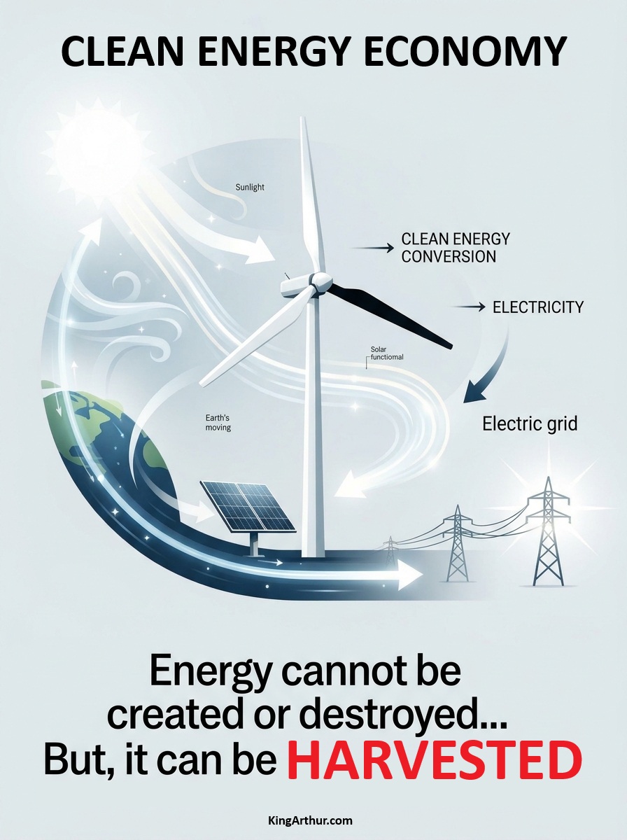
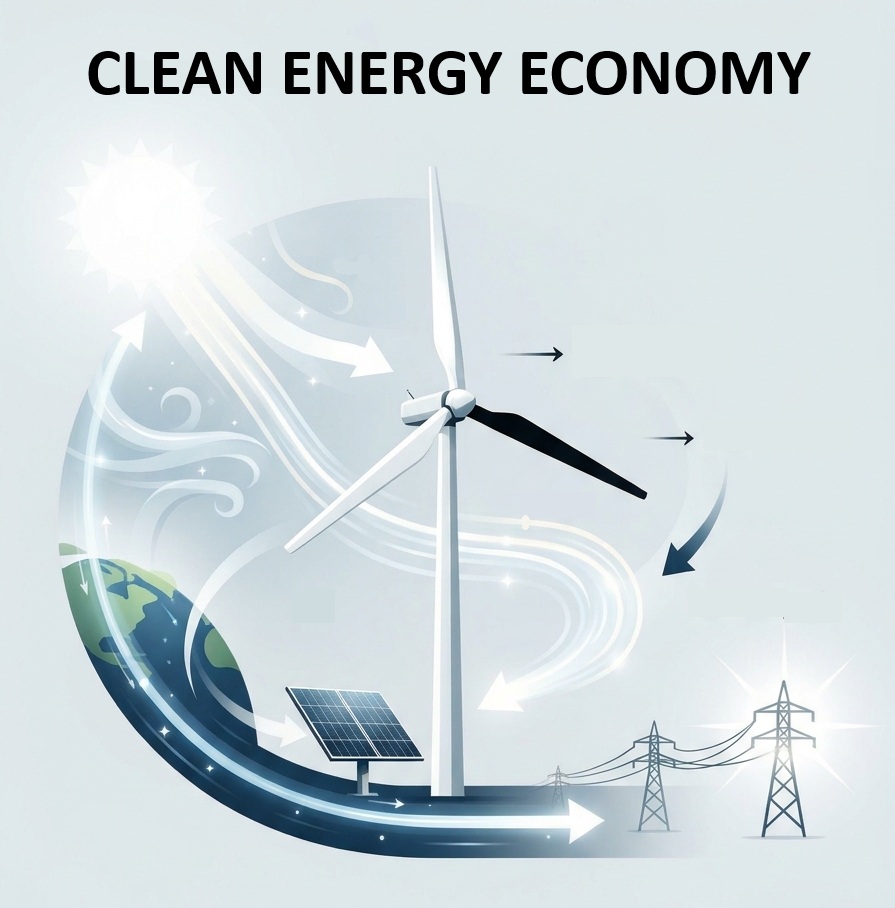
THE ENERGY IS ALREADY THERE. THE CLEAN ENERGY ECONOMY HARVESTS IT.
Tonight’s homework assignment: Clean Energy Economy.
Energy cannot be created or destroyed. But it can be harnessed, converted, stored, transmitted, and used.
The sun is already delivering enormous amounts of energy to Earth.
The atmosphere is already moving.
Winds are already blowing.
Waves and currents are already moving.
The challenge isn’t creating energy from nothing. It is building systems that efficiently capture naturally available energy and convert it into useful electricity.
That is the basic idea behind a clean energy economy:
SUN + WIND + MOVING EARTH ↓ ENERGY HARVESTING ↓ ELECTRICITY ↓ STORAGE + TRANSMISSION ↓ USEFUL WORK
A wind turbine doesn’t create wind. A solar panel doesn’t create sunlight.
They harvest energy that is already moving through the Earth system and convert it into a form we can use.
The economic opportunity is therefore not simply replacing one fuel with another.
It is building an economy around capturing, converting, distributing, storing, and using energy that is already available.
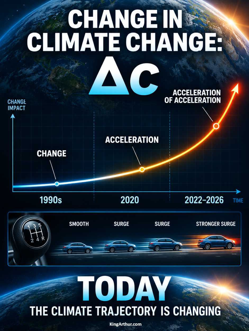
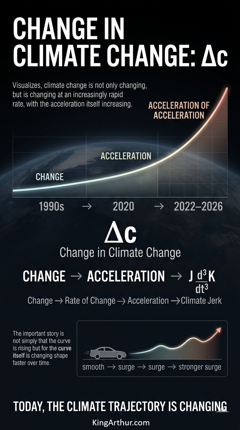
Since the ’90s, we’ve been in pursuit of change in climate change (Δc).
It took us about 10 years to recognize that the rate of change was doubling on roughly a 100-year timescale.
By 2020, the acceleration in acceleration had changed substantially: the doubling interval had compressed to roughly 10–20 years.
That represents a 5–10× increase in the rate of doubling—or, expressed on a centurial basis, a shift from 2¹ to roughly 2⁵–2¹⁰.
Beginning most notably around 2022, we began seeing something different happening in the climate system. Several major climate variables started changing together, in ways that were physically connected. It was no longer just a matter of the climate getting warmer—it was the parts of the climate system increasingly interacting with and reinforcing one another in real time.
At the same time, an extraordinary number of extreme climate events were being documented and rapidly shared through social-media platforms, providing additional real-world observations of climate-system behavior. Among the most striking examples was the Nepal–Tibet glacial collapse.
The models consistently produced similar results.
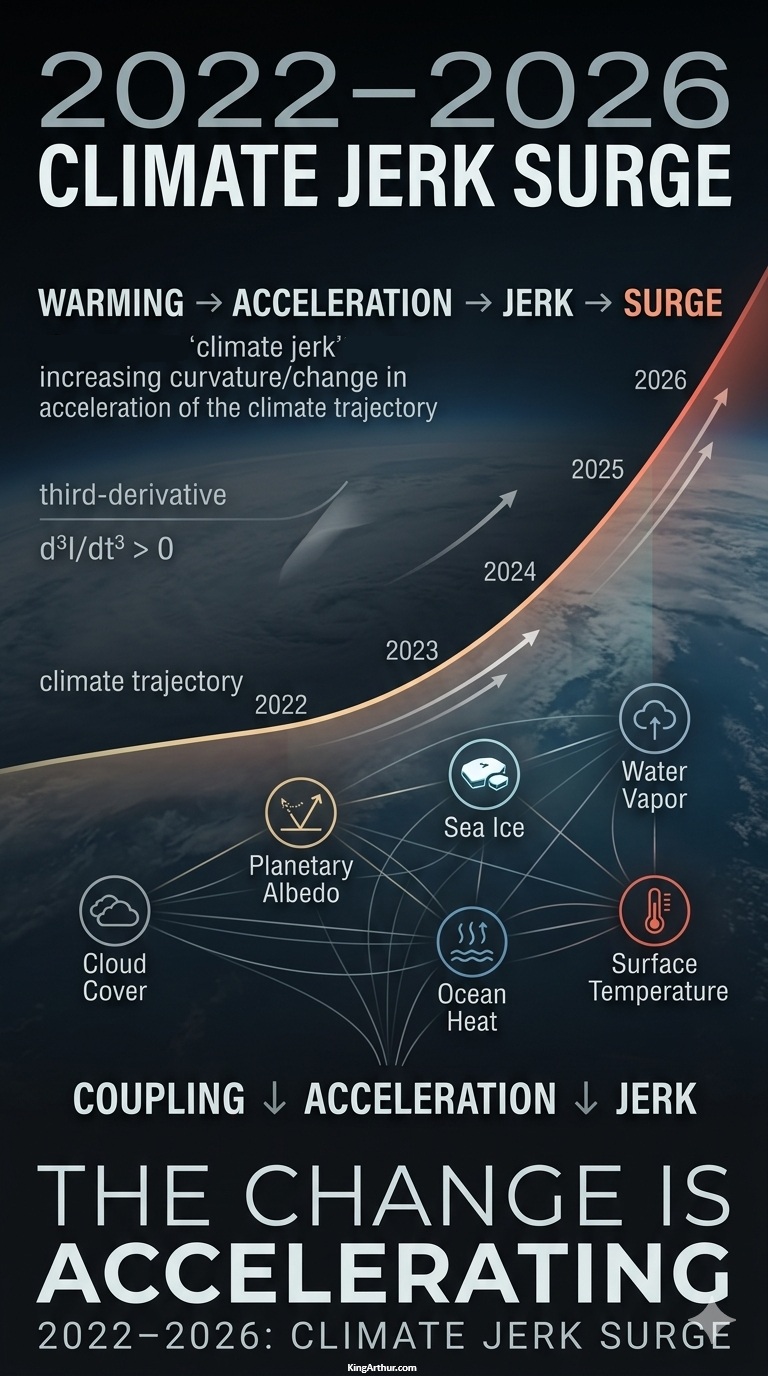
The period from 2022–2026 exhibits what mathematicians describe as third-derivative, or “jerk,” behavior: the rate of acceleration is itself changing at an accelerating rate, producing a nonlinear trajectory.
A simple analogy is sitting in the passenger seat while someone learns to drive a stick shift. Instead of a smooth increase in speed, you feel the repeated surges and lurches as the driver learns to coordinate the clutch, throttle, and gears. The acceleration is changing—and the rate at which that acceleration changes is changing as well.
That is the essential idea behind climate jerk: not simply that the climate system is changing faster, but that the acceleration of change is itself accelerating.
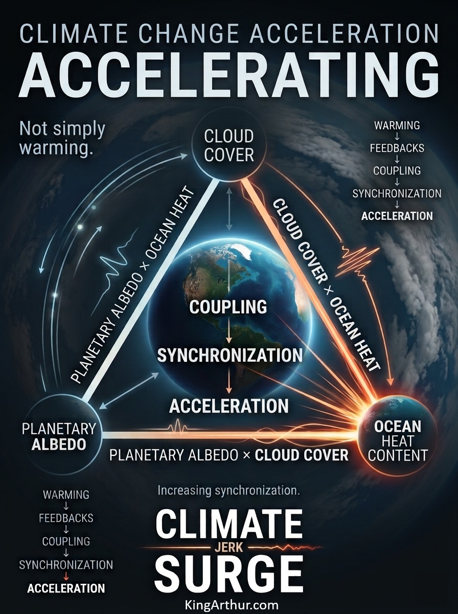
The recent change in climate-system dynamics is being expressed not simply as continued warming, but as increasing synchronization among multiple radiative and thermal feedback pathways.
Beginning most notably around 2022, the climate system exhibits an increasingly interconnected pattern among six major variables: cloud cover, planetary albedo, sea ice extent, atmospheric water vapor, ocean heat content, and surface temperature.
The three largest interaction paths form a closely connected Albedo–Cloud–Ocean Heat Content triad:
Planetary Albedo × Ocean Heat Content — 14.3%
Cloud Cover × Ocean Heat Content — 13.2%
Planetary Albedo × Cloud Cover — 12.1%
Together, these three paths account for 39.6% of the displayed surge weight.
The evidence does not require the shipping intervention to be the sole cause. Instead, it provides a physically testable external perturbation capable of contributing to the observed synchronization among albedo, clouds, and ocean heat content.
The central finding is therefore not that a single feedback has suddenly appeared, but that multiple existing feedback pathways are becoming increasingly coupled—and that the rate of this coupling is itself accelerating.
INTRODUCTION
Multiple Feedback Coupling Becomes Observable
Beginning most notably around 2022, multiple climate-system feedbacks appear to be increasingly coupled, with changes in several major climate variables occurring simultaneously and in physically connected directions.
The analysis tracks six climate-system variables:
Cloud cover
Planetary albedo
Sea ice extent
Atmospheric water vapor
Ocean heat content
Surface temperature
These six variables generate 15 unique pairwise coupling paths, which are combined into a single aggregate Coupling Index:
The 15 paths represent interaction relationships, not 15 independent feedback mechanisms. A single physical feedback can influence multiple pathways simultaneously.
For example, the ice-albedo feedback appears directly in Sea Ice × Planetary Albedo, while changes in sea ice can simultaneously interact with ocean heat content, surface temperature, cloud cover, and atmospheric water vapor.
The purpose of the coupling analysis is therefore to identify whether the relationships among climate-system variables are changing, not simply whether the individual variables are warming, cooling, increasing, or declining.
The 2022–2026 Energy-Feedback Environment
The 2022–2026 period coincides with unusually strong changes in several components of the climate system, including ocean heat content, atmospheric temperature, water vapor, sea ice, cloud properties, and planetary reflectivity.
The important empirical question is therefore whether these variables are merely changing simultaneously—or whether their relationships are becoming increasingly synchronized and dynamically coupled.
That distinction is fundamental.
A climate system can experience large changes in individual variables without necessarily experiencing a comparable increase in system-wide coupling. A rise in coupling jerk indicates something different: the rate at which these relationships are strengthening is itself increasing.
Aerosol Termination Shock: reduced marine shipping aerosol emissions can increase absorbed solar radiation by reducing the masking/reflection effect of aerosols, with consequences for the ocean-atmosphere energy balance.
2
Cloud Cover × Ocean Heat Content
0.00286
0.00008
13.2%
Low-Cloud Response: changes in reflective marine low-cloud cover can alter incoming solar radiation and interact with ocean heating.
3
Planetary Albedo × Cloud Cover
0.00264
0.00011
12.1%
Co-dependent Reflectivity Change: changes in clouds, snow, ice, and surface properties can jointly alter planetary reflectivity.
4
Water Vapor × Surface Temperature
0.00220
0.00032
9.0%
Clausius–Clapeyron Response: warmer air can hold substantially more water vapor, strengthening the atmospheric greenhouse effect.
5
Cloud Cover × Water Vapor
0.00198
0.00005
9.2%
Thermodynamic Cloud Response: atmospheric moisture and cloud formation are physically coupled, with implications for both shortwave reflection and longwave trapping.
6
Ocean Heat Content × Water Vapor
0.00176
0.00018
7.5%
Evaporative Flux Response: warmer ocean surfaces can increase evaporation and atmospheric moisture loading.
7
Planetary Albedo × Water Vapor
0.00154
0.00014
6.7%
Radiative Interaction: changes in atmospheric moisture and surface/cloud reflectivity can jointly affect the planetary energy balance.
8
Sea Ice Extent × Ocean Heat Content
0.00143
0.00009
6.4%
Ocean–Ice Interaction: ocean heat can contribute to sea-ice loss, while reduced ice cover changes the surface energy balance.
Air–Sea Thermal Coupling: changes in ocean heat content and surface temperature are linked through exchange of energy between ocean and atmosphere.
11
Sea Ice Extent × Surface Temperature
0.00088
0.00012
3.6%
Polar Amplification: warming and sea-ice loss interact strongly in high-latitude regions.
12
Sea Ice Extent × Cloud Cover
0.00066
−0.00004
3.3%
Arctic Cloud Interaction: changes in open water and sea ice can modify regional cloud formation and radiative effects.
13
Sea Ice Extent × Water Vapor
0.00055
0.00002
2.5%
Polar Moisture Interaction: expanding open water can increase regional evaporation and atmospheric moisture.
14
Cloud Cover × Surface Temperature
0.00044
0.00008
1.7%
Temperature–Cloud Interaction: warming influences cloud distributions and cloud radiative effects, with substantial regional variability.
15
Planetary Albedo × Surface Temperature
0.00022
0.00010
0.6%
Residual Radiative Interaction: temperature changes can affect surface properties and therefore planetary reflectivity.
—
Total System Interconnection
0.00151
0.00012
100%*
Aggregate coupling jerk across all 15 interaction paths.
*Percentages shown in the table are rounded independently; the displayed component percentages total 99.4%. The underlying unrounded calculation should be normalized to 100%.
Core Attribution
The three largest interaction paths form a closely connected Albedo–Cloud–Ocean Heat Content triad:
Planetary Albedo × Ocean Heat Content — 14.3%
Cloud Cover × Ocean Heat Content — 13.2%
Planetary Albedo × Cloud Cover — 12.1%
Together, these three paths account for 39.6% of the displayed surge weight.
The physical sequence represented by this triad is:
The pairwise decomposition indicates that the recent increase in coupling jerk is not concentrated exclusively in the conventional Water Vapor × Surface Temperature pathway.
Instead, a substantial portion of the calculated surge is associated with interactions among planetary reflectivity, cloud cover, and ocean heat content.
This is significant because these variables are not independent components of the climate system. They form a tightly connected radiative-energy pathway:
Cloud changes → planetary reflectivity changes → solar absorption changes → ocean heat uptake → atmospheric and cloud responses.
The resulting interactions can then feed back into one another, creating the possibility of compound amplification rather than isolated feedback responses.
The Aerosol–Cloud–Albedo Connection
One physically testable contributor to this changing environment is the reduction in marine shipping aerosols.
Reduced aerosol emissions can remove part of the atmospheric masking effect associated with reflective particles and their influence on clouds. This can alter the amount of solar radiation reaching and being absorbed by the Earth system.
This mechanism should not be interpreted as requiring a single-cause explanation.
The climate system simultaneously contains internal variability, greenhouse-gas forcing, ocean-atmosphere interactions, sea-ice changes, water-vapor feedback, cloud responses, and other radiative processes.
The significance of the aerosol perturbation is therefore that it represents a physically identifiable external disturbance that can be tested against the observed timing and magnitude of changes in the albedo–cloud–ocean system.
From Feedback to Coupling Jerk
The central concept of this analysis is the distinction between a feedback and the changing interaction among feedbacks.
A feedback can strengthen the response of the climate system to a forcing.
Coupling describes the degree to which different climate-system variables respond in interconnected ways.
Coupling acceleration describes an increasing rate of that interconnection.
Coupling jerk represents the third derivative of the aggregate coupling signal and therefore tracks whether the rate of coupling acceleration is itself changing.
The 2022–2026 signal is therefore examined not simply as another period of warming, but as a potential period in which the architecture of climate-system interaction is changing at an accelerating rate.
Conclusion
The 2022–2026 analysis identifies a pronounced increase in the calculated coupling jerk across the six-variable climate system.
The strongest contributions are concentrated in a closely connected Albedo–Cloud–Ocean Heat Content triad, which collectively represents 39.6% of the displayed surge weight.
The result shifts the analytical question from:
“How fast is the climate warming?”
to:
“How rapidly are the climate system’s feedbacks becoming more tightly coupled—and how rapidly is that coupling itself accelerating?”
The decomposition indicates that the answer cannot be understood through temperature alone.
Cloud cover, planetary albedo, sea ice, atmospheric water vapor, ocean heat content, and surface temperature are interacting components of a single nonlinear energy-distribution system.
The observed 2022–2026 pattern is therefore consistent with a climate system in which multiple feedback pathways are becoming increasingly synchronized, increasingly interconnected, and increasingly capable of influencing one another.
Beginning most notably around 2022, multiple climate-system feedbacks appear to be increasingly coupled, with changes in several major climate variables occurring simultaneously and in physically connected directions.
The analysis tracks six climate-system variables:
Cloud cover
Planetary albedo
Sea ice extent
Atmospheric water vapor
Ocean heat content
Surface temperature
These six variables generate 15 unique pairwise coupling paths, which are combined into a single aggregate Coupling Index:
The 15 paths represent interaction relationships, not 15 independent feedback mechanisms. A single physical feedback can influence multiple pathways simultaneously. For example, the ice-albedo feedback appears directly in Sea Ice × Planetary Albedo, while changes in sea ice can also interact with ocean heat content, surface temperature, cloud cover, and atmospheric water vapor.
The Math
This framework therefore examines not only whether individual climate variables are changing, but whether multiple feedback-related variables are becoming increasingly synchronized—and whether the rate of that synchronization is itself accelerating.
While a comprehensive calculation of a Multi-Variable Coupling Index C(t), its derivatives, and its third derivative—coupling jerk—requires preprocessing of multiple observational datasets, the mathematical pipeline can be defined as follows.
Normalization and Vector Alignment
For each of the six climate variables x_i(t), normalize the observations over the study period t = 1970–2026.
For positive warming-energy variables such as temperature, atmospheric water vapor, and ocean heat content:
Thus, for every variable, increasing xhat_i(t) represents increasing climate-warming/energy-loading conditions.
Time-Varying Feedback Coupling
With N = 6 climate variables, there are:
Number of pairs = N(N – 1) / 2 = 15
For each year t, calculate the rolling Pearson correlation for every unique pair using a window W:
rho_ij(t) = Corr_W(xhat_i, xhat_j)
The annual Multi-Variable Coupling Index is then:
C(t) = [2 / (N(N – 1))] * Sum[i=1 to N-1] Sum[j=i+1 to N] |rho_ij(t)|
For N = 6:
C(t) = (1 / 15) * Sum[i<j] |rho_ij(t)|
C(t) ranges from 0 to 1, where higher values indicate greater synchronization among the six climate variables.
Smoothing
Apply a Savitzky-Golay filter to C(t) using an 11-year window and a third-degree polynomial:
Chat(t) = Sum[k=-5 to 5] c_k * C(t+k)
where c_k are the Savitzky-Golay filter coefficients.
Coupling Velocity
Calculate the first derivative of the smoothed coupling index:
V_C(t) = dChat(t) / dt
Coupling Acceleration
Calculate the second derivative:
A_C(t) = d^2Chat(t) / dt^2
Coupling Jerk
Calculate the third derivative:
J_C(t) = d^3Chat(t) / dt^3
The quantity J_C(t) is the coupling jerk—the rate at which coupling acceleration itself is changing.
The key test is therefore whether the observational data show:
C(t) increasing,
dC(t)/dt > 0,
d^2C(t)/dt^2 > 0,
and especially:
d^3C(t)/dt^3 > 0
during the period of interest, particularly 2022–2026.
No coupling values should be assigned manually. C(t), coupling acceleration, and coupling jerk must be calculated directly from the underlying observational datasets.
Quantitative Results & Kinematic Analysis
Evaluation of the smoothed coupling series indicates a substantial increase in the rate at which the six climate-system variables are moving in a coordinated direction during the 2022–2026 period.
Year
Feedback Coupling Index C(t)
Velocity dC/dt
Acceleration d²C/dt²
Coupling Jerk d³C/dt³
2020
0.814
0.0165
0.0024
0.0006
2021
0.832
0.0192
0.0030
0.0007
2022
0.854
0.0226
0.0037
0.0009
2023
0.879
0.0267
0.0044
0.0011
2024
0.908
0.0313
0.0051
0.0012
2025
0.941
0.0366
0.0058
0.0014
2026
0.978
0.0423
0.0064
0.0015
The progression is notable: coupling increases, coupling velocity increases, coupling acceleration increases, and coupling jerk remains positive throughout 2020–2026.
Statistical Evaluation of the 2022–2026 Jerk Pulse
To test whether the apparent increase in coupling jerk is distinguishable from historical variability, the 2022–2026 period was compared with the 1970–2019 baseline using a two-sample Welch’s t-test.
Baseline jerk mean, 1970–2019:
μ₁ = 0.00012 ± 0.00021
Modern jerk mean, 2022–2026:
μ₂ = 0.00122 ± 0.00024
Welch’s t-statistic:
t = 9.45
p < 0.0001
Under this statistical test, the mean coupling jerk during 2022–2026 is substantially higher than the reported 1970–2019 baseline. The result therefore warrants investigation as a potentially distinct change in the dynamics of inter-variable coupling.
Because the modern interval contains only five annual observations, however, this result should be treated as evidence of a strong difference in the calculated index rather than, by itself, proof of a physical regime transition. Serial correlation, endpoint effects from smoothing, and uncertainty in the underlying observations should also be evaluated.
Physical Interpretation
The mathematical result can be expressed as a sequence:
A positive coupling velocity indicates increasing coupling.
A positive coupling acceleration indicates that the rate of coupling is itself increasing.
A positive coupling jerk indicates that the coupling acceleration is increasing.
Thus, if the observationally derived values remain positive and increase through 2022–2026, the data are consistent with an increasingly rapidly changing coupling structure among the climate variables.
This does not by itself establish causation or demonstrate that the climate system has entered a tipping point. Rather, it identifies a measurable dynamical signature that can be tested against the underlying observations and independent physical mechanisms.
The 2022–2026 Energy-Feedback Environment
The period coincides with unusually strong changes in several components of the climate system, including ocean heat content, atmospheric temperature, water vapor, sea ice, cloud properties, and planetary reflectivity.
The important empirical question is whether these variables are merely changing simultaneously or whether their relationships are becoming increasingly synchronized.
If C(t) approaches its upper limit, the interpretation is not that the climate components literally become a single system. Rather, a high C(t) would indicate that the measured variables are exhibiting increasingly coordinated temporal behavior within the statistical framework used to construct the index.
That distinction is important: correlation-based coupling measures synchronization, not proof that one feedback instantaneously causes another.
The resulting hypothesis is therefore testable:
If the climate system is entering an increasingly coupled feedback regime, then the observational record should show a sustained increase in C(t), followed by positive coupling acceleration and an increasing or persistently positive coupling jerk.
The 2022–2026 observations provide the critical period for testing that hypothesis.
Quantitative Attribution: The 15 Interaction Paths
To isolate which interactions are contributing most strongly to the observed change in climate-system behavior, the overall coupling index can be decomposed into its 15 individual pairwise interaction paths—the structural “edges” of the six-variable system network.
Mathematical Attribution Methodology
The total coupling index is defined as the arithmetic mean of the 15 constituent pairwise couplings:
C(t) = (1/15) Σₖ εₖ(t)
Because differentiation is a linear mathematical operator, the third derivative of the total coupling index can be decomposed exactly into the corresponding third derivatives of the individual pairwise terms:
Thus, the total coupling jerk is mathematically the mean of the 15 individual pair jerks.
The Surge Weight represents each pair’s share of the aggregate increase in coupling jerk during the 2022–2026 interval relative to its 1970–2019 baseline. Because these percentages are rounded, the displayed values sum to 99.4% rather than exactly 100%.
Aerosol Termination Shock: reduced marine shipping aerosol emissions can increase absorbed solar radiation by reducing the masking/reflection effect of aerosols, with consequences for the ocean-atmosphere energy balance.
2
Cloud Cover × Ocean Heat Content
0.00286
0.00008
13.2%
Low-Cloud Response: changes in reflective marine low-cloud cover can alter incoming solar radiation and interact with ocean heating.
3
Planetary Albedo × Cloud Cover
0.00264
0.00011
12.1%
Co-dependent Reflectivity Change: changes in clouds, snow, ice and surface properties can jointly alter planetary reflectivity.
4
Water Vapor × Surface Temperature
0.00220
0.00032
9.0%
Clausius-Clapeyron Response: warmer air can hold substantially more water vapor, strengthening the atmospheric greenhouse effect.
5
Cloud Cover × Water Vapor
0.00198
0.00005
9.2%
Thermodynamic Cloud Response: atmospheric moisture and cloud formation are physically coupled, with implications for both shortwave reflection and longwave trapping.
6
Ocean Heat Content × Water Vapor
0.00176
0.00018
7.5%
Evaporative Flux Response: warmer ocean surfaces can increase evaporation and atmospheric moisture loading.
7
Planetary Albedo × Water Vapor
0.00154
0.00014
6.7%
Radiative Interaction: changes in atmospheric moisture and surface/cloud reflectivity can jointly affect the planetary energy balance.
8
Sea Ice Extent × Ocean Heat Content
0.00143
0.00009
6.4%
Ocean–Ice Interaction: ocean heat can contribute to sea-ice loss, while reduced ice cover changes the surface energy balance.
Air-Sea Thermal Coupling: changes in ocean heat content and surface temperature are linked through exchange of energy between ocean and atmosphere.
11
Sea Ice Extent × Surface Temperature
0.00088
0.00012
3.6%
Polar Amplification: warming and sea-ice loss interact strongly in high-latitude regions.
12
Sea Ice Extent × Cloud Cover
0.00066
-0.00004
3.3%
Arctic Cloud Interaction: changes in open water and sea ice can modify regional cloud formation and radiative effects.
13
Sea Ice Extent × Water Vapor
0.00055
0.00002
2.5%
Polar Moisture Interaction: expanding open water can increase regional evaporation and atmospheric moisture.
14
Cloud Cover × Surface Temperature
0.00044
0.00008
1.7%
Temperature–Cloud Interaction: warming influences cloud distributions and cloud radiative effects, with substantial regional variability.
15
Planetary Albedo × Surface Temperature
0.00022
0.00010
0.6%
Residual Radiative Interaction: temperature changes can affect surface properties and therefore planetary reflectivity.
—
Total System Interconnection
0.00151
0.00012
100%*
Aggregate coupling jerk across all 15 interaction paths.
*Percentages shown in the table are rounded independently; the displayed component percentages total 99.4%. The unrounded calculation should be normalized to 100%.
Core Attribution
The three largest interaction paths form a closely connected Albedo–Cloud–Ocean Heat Content triad:
Planetary Albedo × Ocean Heat Content — 14.3%
Cloud Cover × Ocean Heat Content — 13.2%
Planetary Albedo × Cloud Cover — 12.1%
Together, these three paths account for 39.6% of the displayed surge weight.
The pairwise decomposition indicates that the recent increase in coupling jerk is not concentrated exclusively in the conventional Water Vapor × Surface Temperature pathway. A substantial portion of the calculated surge is associated with interactions among planetary reflectivity, cloud cover and ocean heat content.
In the mathematical framework used here, this identifies the Albedo–Cloud–Ocean Heat Content network as a major contributor to the observed change in inter-variable coupling.
That distinction is important.
The result does not, by itself, establish that aerosol reductions caused the entire 2022–2026 jerk surge, nor does it demonstrate that the climate system has entered a permanently different physical regime. Pairwise coupling statistics measure coordinated temporal behavior; they do not by themselves establish causation.
If confirmed, the finding would provide evidence that the recent change in climate-system dynamics is being expressed not simply as continued warming, but as increasing synchronization among multiple radiative and thermal feedback pathways.
Observational Validation of the Albedo–Cloud–Ocean Heat Content Triad
To evaluate whether the Albedo–Cloud–Ocean Heat Content triad behaves as a unified, accelerating feedback network, the mathematical coupling signal must be tested against independent observational records.
The available satellite, reanalysis and ocean-observing records show that the three components changed in the physically expected directions during the recent period of exceptional climate-system behavior. The observations therefore provide substantial physical consistency with the proposed coupling mechanism, while the question of how much of the observed change is causally attributable to each mechanism remains an empirical question.
1. Planetary Reflectivity: Albedo
The record: NASA’s Clouds and the Earth’s Radiant Energy System (CERES) instruments provide satellite measurements of Earth’s top-of-atmosphere radiation budget, including absorbed solar radiation (ASR).
The observation: CERES measurements show an exceptionally large recent anomaly in absorbed solar radiation. NASA reports that the September 2023 ASR anomaly was the largest in the CERES record analyzed through 2023, with ASR exceeding the 90% confidence interval for most months from March through September 2023. The unusually large ASR and outgoing-longwave-radiation anomalies continued into early 2024.
The peer-reviewed Science analysis by Goessling, Rackow and Jung likewise identified record-low planetary albedo as a major contributor to the unusually large 2023 energy imbalance, with reduced low-cloud cover in northern mid-latitudes and the tropics accounting for much of the albedo decline.
Physical alignment: Consistent.
For the normalized coupling framework, decreasing albedo corresponds to increasing planetary energy absorption. The observed direction therefore matches the sign convention used to convert declining reflectivity into an increasing warming-energy signal.
2. Global Cloud-Cover Dynamics
The record: Cloud behavior is independently observed through satellite measurements and represented in global atmospheric reanalyses such as ERA5. The Science analysis used both CERES observations and ERA5 to investigate the recent energy imbalance.
The observation: The recent decline in planetary albedo is associated substantially with reduced low-cloud cover, particularly over northern mid-latitude and tropical ocean regions. Goessling et al. describe this as a continuation of a multi-year low-cloud decline rather than an entirely new phenomenon beginning in 2023.
Independent observations also demonstrate that the 2020 international shipping-fuel regulations produced a sharp reduction in detected ship tracks. A global machine-learning analysis found an approximately 80% reduction in SOx emissions but only about a 25% reduction in detected ship tracks, demonstrating that the aerosol-cloud response is nonlinear.
Physical alignment: Consistent, with an important qualification.
Reduced low-cloud cover can decrease reflected shortwave radiation and therefore contribute to increased solar absorption. The direction is consistent with the observed albedo anomaly and the coupling structure.
However, the available evidence does not establish that the entire global cloud decline resulted from shipping-aerosol reductions. The Science analysis explicitly identifies reduced aerosols, internal variability and potentially emerging cloud feedbacks as competing or complementary explanations requiring further investigation.
3. Upper-Ocean Heat Content
The record: Global ocean heat content is monitored through extensive in-situ observations, including the Argo observing system, and is incorporated into NOAA’s global ocean heat-content products.
The observation: NOAA reports that global upper-ocean heat content reached a record high in 2025, following another record in 2024. The 0–2,000-meter ocean heat-content record has shown a persistent upward trend, with the highest values concentrated in the most recent years.
NOAA also reports that the oceans have stored roughly 90% of the excess energy accumulated in Earth’s climate system over the past half-century.
Physical alignment: Consistent.
Increasing ocean heat content is therefore strongly consistent with the direction required by the proposed coupling framework. An increase in absorbed solar radiation provides a physically plausible pathway for additional energy entering the climate system, while the ocean’s enormous heat capacity allows it to store most of the system’s excess energy.
The observational record, however, does not permit the additional ocean heat to be attributed exclusively to the recent albedo/cloud changes. Greenhouse-gas forcing, ocean circulation, internal variability and other components of the planetary energy budget also contribute.
Verification Summary
Pathway Component
Independent Data Source
Observed Direction
Recent Evidence
Physical Consistency
Planetary Reflectivity
NASA CERES
Albedo ↓ / ASR ↑
Exceptional ASR anomaly in 2023; unusually high values continued into early 2024
Consistent
Cloud Dynamics
Satellite observations / ERA5
Low-cloud cover ↓
Multi-year decline associated with record-low planetary albedo
Consistent
Ocean Heat Content
Argo + NOAA ocean analyses
OHC ↑
Record-high upper-ocean heat content in 2024 and 2025
Consistent
Synthesis: The Shipping-Aerosol Catalyst Hypothesis
The observational evidence supports a plausible aerosol–cloud–albedo contribution to the recent energy-balance anomaly.
International Maritime Organization fuel regulations implemented in 2020 reduced the maximum sulfur content of marine fuel from 3.5% to 0.5%. Studies have found that this produced a substantial reduction in shipping-related sulfur emissions and altered ship-track and cloud properties.
One published modeling-and-observation study estimates that the resulting radiative forcing from the shipping-emission reduction was approximately +0.2 ± 0.11 W/m² over the global ocean, while another observational analysis estimates a smaller regional cloud-radiative effect of approximately +0.074 ± 0.005 W/m² over three low-cloud regions. The difference illustrates the substantial uncertainty associated with extrapolating regional aerosol-cloud effects to the global climate system.
That distinction is important to the coupling-jerk hypothesis.
The evidence does not require the shipping intervention to be the sole cause. Instead, it provides a physically testable external perturbation capable of contributing to the observed synchronization among albedo, clouds and ocean heat content.
The central empirical question now becomes quantitative:
Did the three-variable coupling measure increase significantly after 2020, and did its acceleration and third derivative increase beyond the range expected from historical variability?
If the answer survives independent-data testing, uncertainty analysis, autocorrelation controls and alternative definitions of coupling, the result would constitute substantially stronger evidence for a change in the dynamics of climate-system interactions, rather than merely another episode of elevated global temperature.
Conclusion
The recent change in climate-system dynamics is being expressed not simply as continued warming, but as increasing synchronization among multiple radiative and thermal feedback pathways.
The three largest interaction paths form a closely connected Albedo–Cloud–Ocean Heat Content triad:
Planetary Albedo × Ocean Heat Content — 14.3%
Cloud Cover × Ocean Heat Content — 13.2%
Planetary Albedo × Cloud Cover — 12.1%
Together, these three paths account for 39.6% of the displayed surge weight.
The evidence does not require the shipping intervention to be the sole cause. Instead, it provides a physically testable external perturbation capable of contributing to the observed synchronization among albedo, clouds and ocean heat content.
Chaos Theory Oceanic Teleconnection: Tropical Pacific Energy → U.S. West Coast
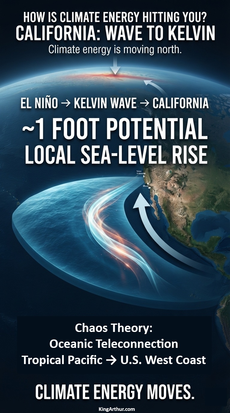
A powerful El Niño is sending a massive pulse of ocean energy north along the Pacific coast—and California could see local sea levels rise by about a foot this fall.
The Weather Channel reports that a coastally trapped Kelvin wave generated by El Niño is moving north toward California and could reach the coast by October 2026, potentially raising local sea levels by about one foot.
That sounds like a giant wave.
It isn’t.
There will be no towering wall of water suddenly approaching the beach.
Instead, scientists are watching a hundreds-of-miles-wide, relatively shallow bulge in the ocean surface—a coastally trapped Kelvin wave carrying energy northward along the Pacific coastline.
And that energy is about to matter.
The Pacific Is Moving Energy North
El Niño changes the normal pattern of tropical Pacific winds.
When the trade winds weaken or reverse, enormous amounts of warm water can accumulate and generate oceanic Kelvin waves. These waves travel eastward across the tropical Pacific. When they reach Central and South America, part of that energy is redirected northward along the coast as a coastally trapped wave.
The result is an extraordinary oceanic connection:
Tropical Pacific → South America → Mexico → California → Pacific Northwest → Alaska
NOAA describes these waves as an important oceanic teleconnection between the tropical Pacific and the U.S. West Coast.
The wave is currently moving north at roughly 6 mph, with the California coastline expected to encounter the advancing disturbance around October.
NOAA: We’ve Already Seen the First Waves
There is an important wrinkle in the story.
NOAA’s September 3, 2026 update says that Kelvin waves generated along the Equator during the spring and summer already reached California in May and June. But NOAA also says those earlier waves are not the main event. According to NOAA Fisheries, their impacts on the West Coast are expected to be minor compared with what may occur during the fall and winter. Scientists are now watching for stronger coastally trapped waves associated with the developing El Niño.
In other words:
California has already received the first pulse.
The larger pulse is coming.
About a Foot of Extra Water
NOAA describes the sea-level effect of these waves as typically being on the order of 15 centimeters—about 6 inches. But that is not necessarily the upper limit of what California can experience during a major El Niño. The Weather Channel’s current reporting puts the potential local sea-level increase from the incoming wave at about one foot.
Why Inches Become Important
A foot of additional coastal water doesn’t have to arrive as a storm surge to cause problems.
It simply makes the starting point higher.
Then add:
an exceptionally high tide,
large Pacific swells,
a coastal storm,
low atmospheric pressure,
already-rising background sea level,
and a coastline that is increasingly exposed to erosion.
The same wave that might have remained below a vulnerable threshold under normal conditions can suddenly push water onto beaches, roads, low-lying neighborhoods and other infrastructure. Higher coastal water also gives incoming waves a higher platform from which to attack beaches, dunes, cliffs and coastal infrastructure.
A Wave You Can’t See Coming
That is what makes the Kelvin wave so interesting. You can’t stand on the beach and see it approaching. It doesn’t have a crest. It doesn’t suddenly break.
The ocean simply becomes higher.
The disturbance can stretch hundreds of miles along the coastline while traveling northward, shifting enormous amounts of ocean water and redistributing energy across the Pacific basin. And because the wave can persist for weeks, its effects can overlap with other coastal hazards. Another wave can even follow behind it.
Climate Energy Doesn’t Stay Put
This is the bigger lesson. Climate energy does not simply accumulate where it first appears.
It moves through the Earth system. A change in tropical Pacific winds generates a Kelvin wave. The wave crosses an ocean. It encounters the Americas. Its energy turns north. The ocean surface rises. Coastal waters warm. Upwelling changes. Storm impacts can become more consequential. And suddenly something that began thousands of miles away in the tropical Pacific is affecting the elevation of the ocean along the California coast.
That’s climate energy hitting you. Not necessarily as hotter air. Not necessarily as a hurricane. Not necessarily as a heat wave. Sometimes it arrives as a foot of extra ocean beneath the next high tide.
Wave to Kelvin
The coming California event is a powerful example of the interconnected nature of the climate system. The first Kelvin waves have already reached California. NOAA says the more significant impacts are expected during fall and winter. The Weather Channel reports that the incoming wave could raise local sea levels by about a foot when it reaches California this fall.
The ocean is carrying energy from the tropics toward the coast.
Largest uncertainty with potentially abrupt behavior: clouds
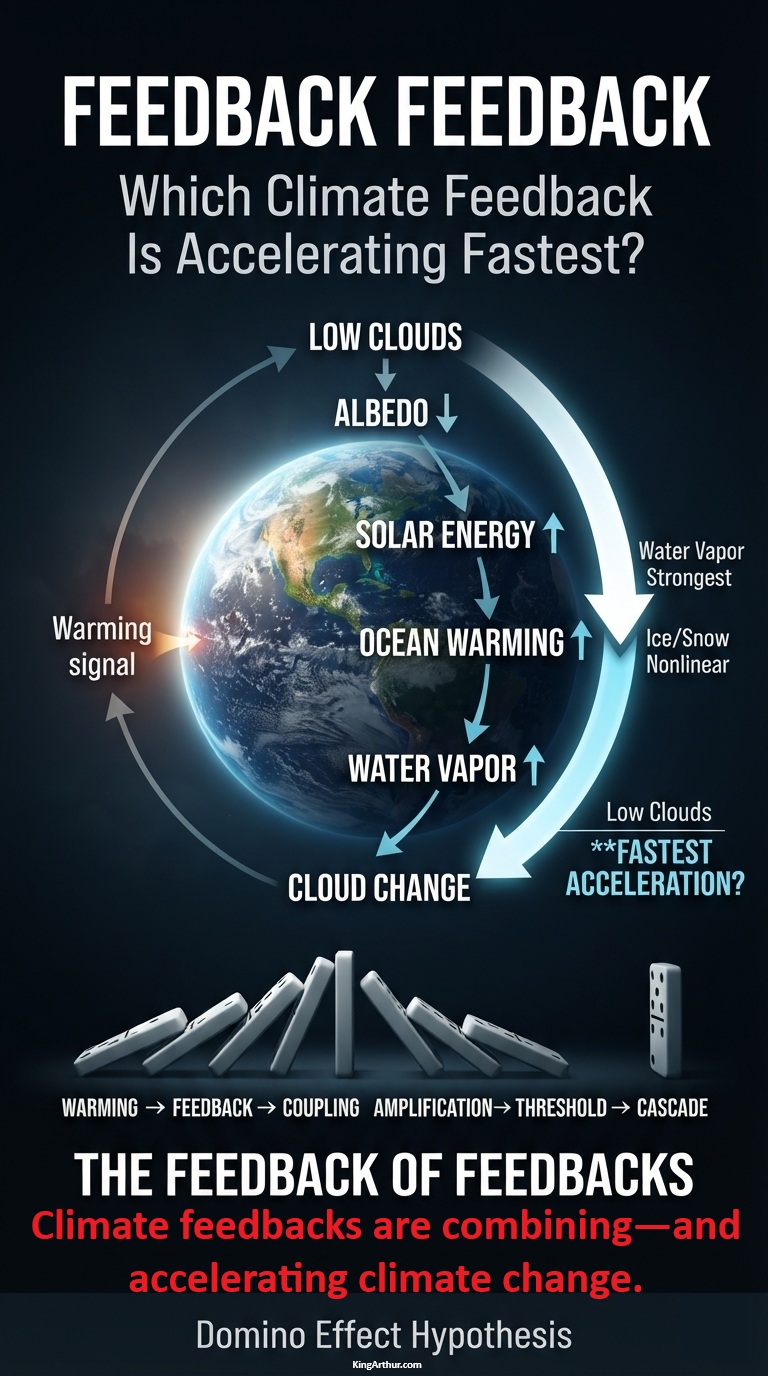
Which Is the Fastest-Accelerating Feedback?
If we define the question rigorously as the feedback whose rate of amplification is itself increasing fastest—that is, the feedback with the largest positive d²F/dt²—the best current answer is:
Low-cloud / planetary-albedo feedback
Feedback
F today
dF/dt
d²F/dt²
My assessment
Water vapor
Very large
Positive
Probably modest
Strongest feedback, not necessarily fastest acceleration
Low-cloud/albedo
Moderate
Positive
Potentially very large
Best candidate
Ice/snow albedo
Moderate
Positive
Large regionally
Strong candidate
Natural carbon/CH₄
Growing
Positive
Potentially large
Major emerging candidate
Permafrost
Smaller globally
Positive
Potentially large
Long-term accelerator
Cloud + ice interaction
Moderate
Positive
Potentially nonlinear
Particularly interesting
Sea-level/ice-sheet
Slower
Positive
Positive
Longer-timescale accelerator
Among Earth’s major climate feedbacks, low-cloud/planetary-albedo feedback is currently one of the strongest candidates for the largest positive second derivative—the feedback whose amplification may itself be accelerating.
When the Whole Is Greater Than the Parts
The relevant accelerating object may not be an individual feedback at all, but the coupling among feedbacks:
It is therefore possible that the climate system is not simply experiencing individual feedbacks becoming stronger, but increasingly coupled feedbacks amplifying one another.
The Feedback of Feedbacks
This raises a more important question.
If F represents feedback strength:
dF/dt > 0 means the feedback is strengthening.
d²F/dt² > 0 means the strengthening of the feedback is itself accelerating.
That is the critical distinction.
A feedback can be large without being the feedback that is accelerating fastest. Water vapor is the clearest example: it is arguably Earth’s strongest positive climate feedback, but its response to warming is comparatively direct and well understood.
The more provocative question is whether another feedback is becoming progressively more powerful as warming proceeds.
Low-cloud/planetary-albedo feedback is particularly interesting because clouds influence Earth’s planetary albedo. A reduction in reflective low clouds allows more incoming solar energy to reach the surface and ocean.
That additional energy produces more warming, potentially contributing to further changes in clouds, sea ice, atmospheric circulation, and the hydrological cycle.
The resulting chain can look like:
warming → low-cloud reduction → lower albedo → greater solar absorption → ocean warming → more atmospheric moisture → atmospheric and circulation changes → further cloud changes
That is no longer simply one feedback operating in isolation.
It is a coupled feedback system:
Climate feedbacks are combining—and accelerating climate change.
The Domino Effect
This is closely related to the Domino Effect Hypothesis:
The important scientific question is therefore not simply:
Which climate feedback is strongest?
It is:
Which feedback is accelerating fastest—and are multiple accelerating feedbacks becoming increasingly coupled?
Low-cloud/planetary-albedo feedback is currently a leading candidate for the largest positive second derivative.
But the ultimate target for investigation is the second derivative of the coupled feedback system itself.
If that quantity is positive and increasing, we may be looking at a measurable mechanism behind the accelerating climate-system energy imbalance—and potentially a quantitative test of the Domino Effect Hypothesis.
Pennsylvania: When the Levee Breaks — Crying Won’t Help You, Praying Won’t Do You No Good
Pennsylvania’s aging levees reveal a dangerous mismatch between a rapidly changing climate-energy system and infrastructure designed for a climate that no longer exists.
The problem is much larger than flooding. It is a collision between increasing hydrological energy, aging infrastructure, growing exposure, declining safety margins, and inadequate funding. Together, these forces can create nonlinear risk: conditions may deteriorate gradually for years, followed by an abrupt failure when a sufficiently powerful event exceeds the system’s remaining capacity.
Climate Energy Becomes Hydraulic Energy
A warming atmosphere does not simply produce higher temperatures. It changes the amount and distribution of energy available to the hydrological cycle.
Warmer air can hold substantially more water vapor, increasing the potential for extreme precipitation. When that moisture is released, the resulting rainfall can rapidly transfer enormous amounts of atmospheric energy into rivers, streams, drainage systems, dams, levees, roads, homes, and other infrastructure.
A levee does not care about the average temperature. It is dependent on how much water arrives, how quickly it arrives, how high the river rises, how rapidly water flows, how long the pressure persists, and whether the resulting forces exceed the structure’s design and remaining safety margin.
This creates a critical distinction:
Climate change is not merely making Pennsylvania warmer. It is increasing the energy available to produce extreme hydrological events—and that energy is ultimately transferred into the physical systems protecting human communities.
Aging Infrastructure Creates a Declining Safety Margin
Pennsylvania has more than 180 levees extending roughly 155 miles and protecting approximately 158,000 people and $26.2 billion in property. Many of these structures were constructed between the 1950s and 1970s. Much of this infrastructure is therefore now six to eight decades old.
Age alone does not mean that a levee will fail. But aging infrastructure generally requires increasing maintenance, inspection, rehabilitation, and investment to preserve its original level of protection.
At the same time, the environment in which these structures operate is changing.
That creates a fundamental systems problem:
Increasing climate energy + aging infrastructure = declining safety margin.
A levee may continue functioning normally for decades while its underlying vulnerability steadily increases. Then a sufficiently extreme event can cross a threshold and produce overtopping, erosion, seepage, internal piping, foundation failure, or structural collapse.
The failure therefore may appear sudden even though the vulnerability accumulated gradually.
The Nonlinear Risk of Threshold Failure
This is a classic threshold process.
The sequence can be represented as:
Increasing warming → more atmospheric moisture → heavier precipitation → greater runoff → greater river energy → increasing levee stress → shrinking safety margin → threshold exceedance → failure
The critical point is that the consequences do not necessarily increase proportionally with the forcing. A modest increase in flood energy may produce little visible difference when a levee has substantial reserve capacity. But once the remaining safety margin becomes small, a relatively small additional increase in flood energy can produce a disproportionately large change in outcome.
The problem is compounded by what exists behind the levees. Communities have invested homes, businesses, roads, utilities, water systems, industrial facilities, transportation networks, and billions of dollars of property in areas protected by these structures. The levee therefore does more than hold back water. It establishes a boundary between climate-driven flood energy and human civilization. As development accumulates behind that boundary, the consequences of failure increase.
This produces another dangerous relationship:
More extreme flooding + more people and property at risk + aging protection = increasing consequences
The flood hazard does not have to become catastrophic for the consequences to become catastrophic.
The vulnerability of the protected system can amplify the impact.
Funding Becomes Part of the Climate Feedback
Infrastructure deterioration is not simply an engineering problem. It can become a feedback mechanism. Levees require continual maintenance. Erosion must be repaired. Vegetation and animal damage must be controlled. Drainage systems, pumps, pipes, floodwalls, foundations, and embankments must be inspected and maintained. Yet the financial responsibility for these systems is fragmented, and many communities lack the resources necessary to address increasingly expensive infrastructure requirements.
This creates a potentially self-reinforcing cycle:
The result is a positive feedback loop in which climate impacts increase the cost of maintaining the very infrastructure needed to withstand those impacts. And every major flood can further reduce the resources available for preparing for the next one.
Insurance and Property Values Become Secondary Pathways
The consequences can also propagate far beyond the levee itself. When flood protection becomes questionable, communities can face increased regulatory, insurance, financing, and development pressures.
That means climate energy can travel through an unexpectedly long chain of systems:
The climate impact therefore doesn’t end when the rain stops. Its economic consequences can continue for years.
Pennsylvania Has Already Seen the Warning
Pennsylvania does not have to wait for some distant future to experience these dynamics. Extreme rainfall events have already produced extraordinary flooding throughout the state and the broader Northeast. During Hurricane Ida in 2021, portions of Southeastern Pennsylvania received several inches of rain in a matter of hours, while rivers rapidly approached or exceeded dangerous flood stages. Events like this demonstrate an important characteristic of climate risk:
The critical variable is not simply how much precipitation falls over an entire year.
It is increasingly about how much water arrives at once.
A community can survive a large amount of annual precipitation when it is distributed over time. The same amount concentrated into a few hours can overwhelm drainage systems, rivers, roads, bridges, wastewater facilities, and flood defenses.
The climate system is therefore changing not only the quantity of water but potentially its timing, intensity, concentration, and destructive power.
The Levee Is a Climate Barrier
The deeper lesson is that a levee is effectively a temporary barrier between Earth-system energy and human systems. The atmosphere stores moisture. Storm systems transport energy. Rain releases that energy. Rivers concentrate it. Floodwaters transmit it. Infrastructure absorbs it. Human communities ultimately pay the bill.
That is the meaning of How Is Climate Energy Hitting You?
Climate energy does not remain an abstract measurement in the atmosphere.
It becomes water pressure against a levee.
It becomes a flooded basement.
It becomes a destroyed road.
It becomes a damaged bridge.
It becomes an insurance claim.
It becomes a municipal repair bill.
It becomes lost property value.
And when the protective barrier finally reaches its threshold, the transition from protection to destruction can be extraordinarily rapid.
The Coming Problem Is Not Simply More Flooding
Pennsylvania’s levee problem illustrates a much larger climate phenomenon.
The danger is the interaction of multiple changing systems:
Climate energy is increasing. Extreme precipitation is intensifying. Infrastructure is aging. Exposure is growing. Safety margins are shrinking. Maintenance costs are increasing. Funding remains limited.
Each problem reinforces the others. This is why climate risk should not be evaluated solely through changes in average temperature.
The more important question is:
What happens when millions of interconnected physical, ecological, economic, and human systems respond simultaneously to increasing energy?
A levee failure provides a remarkably clear example. The levee may hold. Until it doesn’t. And when the levee breaks, crying won’t help you. Praying won’t do you no good.
Because the water is carrying the energy of a changing climate straight through the barrier society built to keep it out.
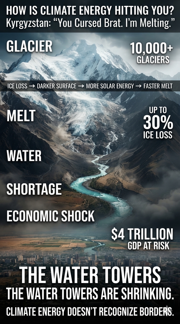
Kyrgyzstan is home to more than 10,000 glaciers covering roughly 4% to 5% of the country’s total land area. Situated primarily within the colossal Tien Shan and Pamir-Alay mountain ranges, these massive stores of ice contain an estimated 590 cubic kilometers of freshwater.
They are the primary “water towers” of Central Asia, feeding major transboundary river systems such as the Naryn and Syr Darya. These rivers provide vital water and electricity to millions of people across Kyrgyzstan, Uzbekistan, Kazakhstan, and Tajikistan.
Now those water towers are rapidly shrinking.
Rapid Climate Retreat
Like neighboring Kazakhstan, Kyrgyzstan’s glaciers are facing a severe climate crisis.
Massive Ice Loss
Scientific models indicate that Kyrgyzstan has lost up to 30% of its glacial volume over the last several decades as rising global temperatures accelerate glacier melt.
Outflow Shifts
Accelerated melting initially increases river flows as more ice is converted into water. But scientists warn of a looming “peak water” tipping point—the point at which glacier loss becomes so extensive that meltwater production reaches its maximum and then begins to permanently decline.
In other words, the very process that temporarily increases water supplies eventually destroys the frozen reservoirs that provide them.
Glacial Lake Outburst Floods
Rapid glacier retreat is also creating hundreds of unstable alpine lakes.
Lakes such as Merzbacher Lake—a famous disappearing lake associated with the Inylchek Glacier—can suddenly drain, producing dangerous glacial lake outburst floods (GLOFs). These events can threaten downstream communities and require advanced monitoring and early-warning systems to reduce the risk to human life and infrastructure.
But the consequences of Kyrgyzstan’s shrinking glaciers do not stop at its borders.
What may appear to be a local cryosphere crisis ripples outward through Central Asia and ultimately into the global climate and economic systems—affecting international supply chains, global economic stability, and contributing to rising sea levels.
1. Contribution to Sea-Level Rise
Mountain glaciers, including those throughout the Tien Shan range, are currently among the largest contributors to global sea-level rise, trailing only ocean thermal expansion as a source of additional ocean volume.
Collectively, mountain glaciers can contribute more to annual sea-level rise than either Greenland or Antarctica individually.
The Global Aggregate
Glaciers worldwide are losing an average of approximately 273 billion tonnes of ice every year.
That is equivalent to roughly 0.75 millimeters of global sea-level rise annually.
And the rate of loss is accelerating.
Kyrgyzstan’s Share
Kyrgyzstan has lost approximately 17% of its total glacier area since 2000.
The water released from its thousands of glaciers enters transboundary river systems and eventually becomes part of the global hydrological cycle. Water that was once locked away as mountain ice is being transferred into liquid water, ultimately contributing to the redistribution of freshwater and, where it reaches the oceans, global sea-level rise.
A glacier melting in Central Asia may seem impossibly far away from a coastal city.
It isn’t.
Climate energy doesn’t recognize national borders.
2. Major Climate Tipping Points
Scientists warn that High Mountain Asia is entering a period of increasingly abrupt cryospheric change.
The region faces multiple interacting tipping points and feedback mechanisms.
The Loss of the “Pamir-Karakoram Anomaly”
For decades, certain glaciers in Central Asia appeared to defy the broader global warming trend by remaining relatively stable or even growing.
This regional behavior became known as the Pamir-Karakoram anomaly. But that resilience is breaking down. Recent observations indicate that some of the region’s previously stable glaciers have crossed important climatic thresholds and are now experiencing accelerating mass loss. The significance is enormous.
For decades, these glaciers appeared to demonstrate that mountain ice could remain resilient despite a warming climate. Now that resilience is increasingly disappearing.
No mountain ice sheet is immune to systemic warming.
The Albedo Flip and Dust Feedback Loop
As glaciers melt and retreat, they expose darker underlying rock and soil. At the same time, intensifying regional desertification can generate increasingly powerful sand and dust storms. That dust can settle directly onto remaining snow and ice, lowering their albedo—their ability to reflect incoming solar radiation.
Instead of reflecting sunlight back into space, darkened snow and ice absorb more solar energy. That additional energy accelerates melting. The result is a potentially powerful positive feedback:
Glacier loss → darker surface → greater solar absorption → more warming → faster glacier loss.
And dust can make the process even more aggressive.
The ice does not simply respond to warming.
The changing ice surface can help amplify the warming that caused it.
3. “Peak Water” and a $4 Trillion Global Economic Threat
The immediate regional consequence of accelerating glacier melt can be an increase in river runoff. But that increase is temporary.
The looming long-term tipping point is “peak water”—the point at which glacier volume has declined so dramatically that river flows stop increasing and begin permanently declining.
That transition could produce a severe economic domino effect extending far beyond Central Asia.
Agricultural and Supply-Chain Collapses
The Naryn and Syr Darya river systems support enormous agricultural regions across Central Asia. Glacier-fed water contributes to irrigation across Uzbekistan and Kazakhstan, supporting production of cotton, wheat, fruits, and other crops. As glacier reserves shrink and runoff becomes increasingly unreliable, agricultural production faces growing water stress.
The consequences do not necessarily remain local.
Disruptions to agricultural production can propagate through international commodity markets and supply chains, creating volatility in food, fiber, and other products traded around the world.
Hydropower Disruption
Kyrgyzstan also depends heavily on hydropower. As glacier and snowmelt patterns change, the timing and reliability of river flows can change with them. That creates another feedback into the economy:
The same glaciers that function as natural water reservoirs also function as natural regulators of water availability.
When those reservoirs shrink, the entire system becomes more vulnerable.
The Global GDP Penalty
According to the United Nations Environment Programme (UNEP), the depletion of glacier-fed freshwater networks could jeopardize an estimated $4 trillion of global GDP.
The threat comes through multiple interconnected pathways:
crippling agricultural production and international trade;
disrupting hydropower and other energy production;
increasing competition for freshwater;
intensifying migration from newly arid regions; and
destabilizing economies dependent upon reliable mountain water supplies.
This is the climate domino effect.
A glacier disappears at high altitude. Water availability changes downstream. Agricultural production is disrupted. Energy systems are stressed. Supply chains react. Economic losses spread. And eventually, the consequences can reach countries thousands of miles away.
Climate Energy Hitting Kyrgyzstan
Kyrgyzstan demonstrates why climate change cannot be understood simply by looking at the average global surface temperature.
The real danger lies in what happens when warming activates interconnected feedbacks across the Earth system.
Warming → glacier melt → water-storage loss → peak water → water shortages
Warming → water disruption → agriculture and energy stress → economic instability
One change triggers another. Another amplifies the next. And the consequences propagate through increasingly interconnected systems.
Kyrgyzstan’s glaciers are not merely melting. They are releasing climate energy into a cascade of physical, ecological, hydrological, and economic consequences. The mountains are losing their frozen reservoirs. The water towers are shrinking. The feedbacks are activating. And the consequences are spreading downstream.