Exposure to extreme heat accelerates biological aging, damaging tissues and shortening telomeres at a cellular level.
Although this article focuses on the current heatwave affecting Philadelphia, the same principles apply across much of the world. As climate change drives more frequent and intense heatwaves, millions of people are facing increasing exposure to dangerous combinations of heat and humidity.
Extreme heat is more than an inconvenience—it is a serious public health hazard. Prolonged exposure can cause heat exhaustion, heatstroke, kidney injury, and cardiovascular stress. Emerging research also indicates that repeated heat stress may accelerate biological aging, impair immune function, increase systemic inflammation, and raise the risk of chronic disease. In the most severe cases, extreme heat can be fatal.
Heatwaves, Wet-Bulb Temperatures, and Human Health: The Growing Threat of Humid Heat
Heat Doesn’t Just Make You Uncomfortable—It Can Age You and Kill You
Extreme humid heat places extraordinary stress on the human body. As global temperatures continue to rise, prolonged heatwaves are becoming more frequent, more intense, and more dangerous. Beyond heat exhaustion and heatstroke, emerging research suggests that chronic exposure to extreme heat accelerates biological aging, increases the burden of chronic disease, and contributes to hundreds of thousands of deaths each year.
Philadelphia is currently experiencing a prolonged and dangerous heatwave. High humidity is driving elevated wet-bulb temperatures, reducing the body’s ability to cool itself through evaporation. Peak wet-bulb temperatures are estimated to reach 79°F to 84°F (26–29°C) in shaded conditions between Wednesday and Friday, with even higher values possible in direct sunlight.
Understanding Wet-Bulb Temperature
Unlike ordinary air temperature, wet-bulb temperature measures the combined effects of heat and humidity. It represents the lowest temperature the body can achieve through evaporative cooling (sweating).
As humidity rises, sweat evaporates less efficiently, making it increasingly difficult for the body to regulate its internal temperature.
Recent physiological and climate-chamber studies indicate that human tolerance is lower than previously believed, particularly during prolonged exposure or physical activity.
Approximate health thresholds include:
Wet-Bulb Temperature
Health Risk
Below 25°C (77°F)
Heat stress is generally manageable with hydration and rest.
25–28°C (77–82°F)
Dangerous for prolonged outdoor work or strenuous exercise.
28–31°C (82–88°F)
Very dangerous. Heat illness becomes increasingly likely, especially for vulnerable populations.
30–33°C (86–91°F)
Healthy individuals may experience rapid heat strain during sustained exposure, direct sunlight, or physical exertion.
Above 31°C (88°F)
Severe risk of heat-related illness, even for healthy adults.
35°C (95°F)
Often cited as the theoretical upper survivability limit under idealized laboratory conditions, although serious health effects occur well below this threshold.
Even below these thresholds, older adults, outdoor workers, children, pregnant women, and individuals with cardiovascular or respiratory disease face substantially elevated risks.
Estimated Wet-Bulb Forecast for Philadelphia
Day
High Temperature
Estimated Peak Wet-Bulb
Monday
89°F (32°C)
72–75°F (22–24°C)
Tuesday
92°F (33°C)
74–77°F (23–25°C)
Wednesday
98°F (37°C)
79–82°F (26–28°C)
Thursday
101°F (38°C)
81–84°F (27–29°C)
Friday
100°F (38°C)
80–84°F (27–29°C)
Saturday
97°F (36°C)
79–82°F (26–28°C)
Sunday
92°F (33°C)
76–79°F (24–26°C)
These values are estimates because wet-bulb temperature varies with hourly changes in humidity, wind speed, cloud cover, and atmospheric pressure.
The current forecast calls for air temperatures approaching or exceeding 100°F (38°C), with heat index values potentially reaching 105–110°F (41–43°C).
Climate Extremes and Cellular Breakdown
Extreme heat affects virtually every organ system in the body.
Recent research indicates that prolonged exposure contributes to:
Heat exhaustion and heatstroke
Severe dehydration
Acute kidney injury
Cardiovascular stress
Worsening respiratory disease
Increased mortality
Emerging biomedical evidence also suggests that repeated heat exposure accelerates biological aging, producing cellular damage associated with shortened telomeres, increased oxidative stress, and impaired DNA repair.
These processes increase long-term risks for diseases including:
Cardiovascular disease
Diabetes
Dementia
Certain cancers
Many of these conditions are further amplified by chronic air pollution and infectious disease.
Heat, Immunity, and Mental Health
Heat stress extends beyond physical illness.
Research increasingly indicates that elevated environmental temperatures contribute to:
Reduced immune efficiency
Increased systemic inflammation
Greater cardiovascular strain
Slower recovery following illness or physical exertion
Accelerated physiological aging
Heat also affects mental health.
Numerous studies have associated prolonged heat exposure with higher rates of:
Anxiety
Depression
Aggression
Sleep disruption
Suicide
These effects become especially pronounced in urban environments where concrete and asphalt absorb heat during the day and release it overnight, preventing normal nighttime cooling.
Heatwaves Create a Dangerous Feedback Loop
Climate change is reinforcing itself through multiple interconnected feedbacks.
One important societal feedback is:
More heat → greater cooling demand → higher electricity consumption → increased emissions (where fossil fuels remain part of the grid) → additional warming → even greater cooling demand.
Breaking this cycle requires both rapid reductions in greenhouse-gas emissions and improvements in energy efficiency, cooling technology, urban planning, and climate adaptation.
The Human Limit
For decades, climate discussions focused primarily on environmental impacts. Increasingly, however, human physiology is becoming one of the defining constraints of climate change.
The ability of the human body to dissipate heat ultimately determines where people can safely work, exercise, and even survive.
As humid heat becomes more common, understanding wet-bulb temperatures is no longer simply a matter of meteorology—it is becoming central to public health, infrastructure planning, labor productivity, emergency management, and climate policy.
The challenge of the twenty-first century is no longer simply preventing additional warming. It is adapting to a climate in which human heat tolerance itself is becoming one of Earth’s most important limiting factors.
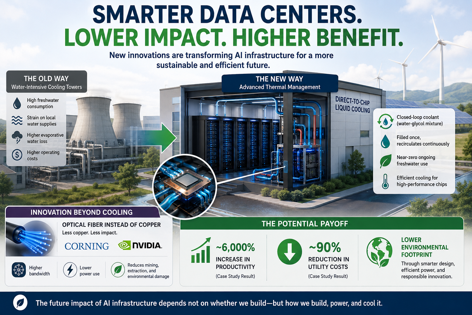
New data center designs are dramatically reducing—or in some cases eliminating—direct freshwater consumption by replacing traditional, water-intensive cooling towers with advanced thermal management technologies. Major technology companies and hardware manufacturers are rapidly deploying infrastructure designed to minimize strain on local water supplies while supporting rapidly growing computational demand.
One of the most significant developments is the adoption of modern direct-to-chip liquid cooling systems. These systems use a closed-loop coolant, typically a water-glycol mixture, which is filled once during installation and then continuously recirculated. Because the coolant is reused within a sealed system, these designs require little to no ongoing freshwater input while still efficiently removing heat from high-performance processors.
As these technologies become more widespread, it is important to recognize that blanket opposition to AI or new data centers may unintentionally slow the deployment of infrastructure that is substantially more water- and energy-efficient than earlier generations. The environmental impact of data centers depends less on their existence and more on how they are designed, powered, and cooled.
Beyond cooling systems, there are additional innovations shaping the next generation of AI infrastructure that are often overlooked. One example is the gradual replacement of copper interconnects with optical fiber. Companies such as Corning are partnering with Nvidia to introduce advanced optical networking within AI data centers. This transition significantly reduces reliance on copper, which has downstream implications for mining, extraction, and other environmentally intensive industrial processes. In turn, this shift has the potential to lower the broader ecological footprint associated with large-scale computing infrastructure.
The reason I’m outspoken on this issue is that the potential benefits of AI and modern data centers can far outweigh their costs when they’re deployed responsibly. In my work as an economist and climate scientist, I have documented a case study indicating approximately a 6,000% increase in productivity alongside a reduction of roughly 90% in utility costs under modernized systems and workflows.
That doesn’t mean every AI deployment is beneficial or that environmental concerns should be ignored. It does mean we should evaluate these technologies based on current evidence and engineering advances, rather than broad, generalized claims that treat all AI and all data centers as inherently harmful.
Addendum: A Case Study in AI Efficiency
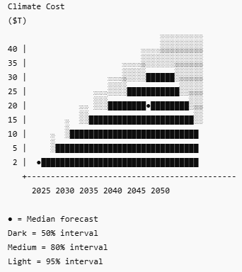
As an economist and climate scientist, I’ve been experimenting with different AI graphic generators to evaluate them from both a marketing and an economic perspective. My objective is simple: maximize impact while minimizing cost and environmental footprint.
Rather than focusing solely on image quality, I compare the complete cost-benefit equation, including environmental resource use, computational efficiency, human labor, production time, and audience response. My goal is to identify which tools produce the greatest overall value.
My current comparison has focused primarily on ChatGPT and Google’s Nano Banana image generator. Thus far, ChatGPT has proven to be slightly more computationally expensive but often produces graphics with greater visual impact. Nano Banana, on the other hand, tends to generate a cleaner, more formal aesthetic that may resonate better with certain audiences. Both systems have strengths, and each may be the better choice depending on the intended purpose.
What surprised me most was not how difficult it was to generate the images, but how easy it became once the underlying work had been completed. The challenging part was researching the subject, writing the paper, and translating complex scientific concepts into a clear set of instructions for the AI. Once those instructions existed, both systems produced high-quality graphics in well under a minute.
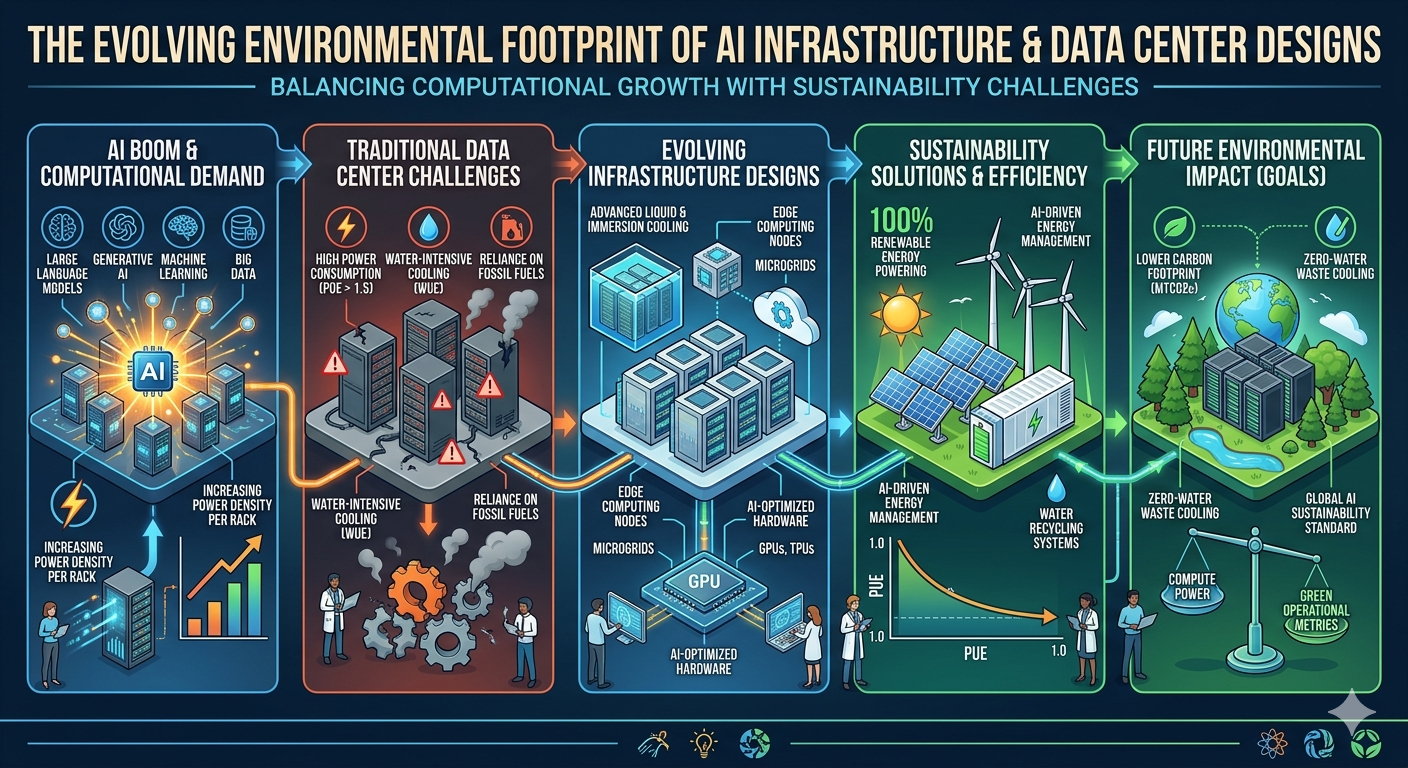
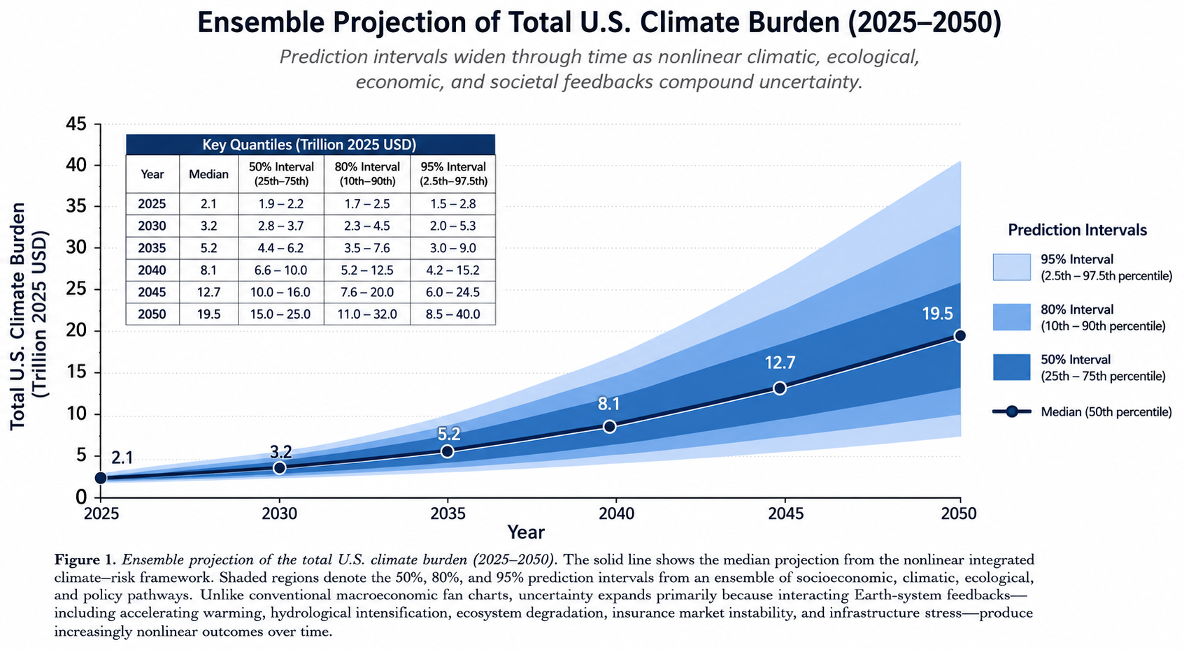
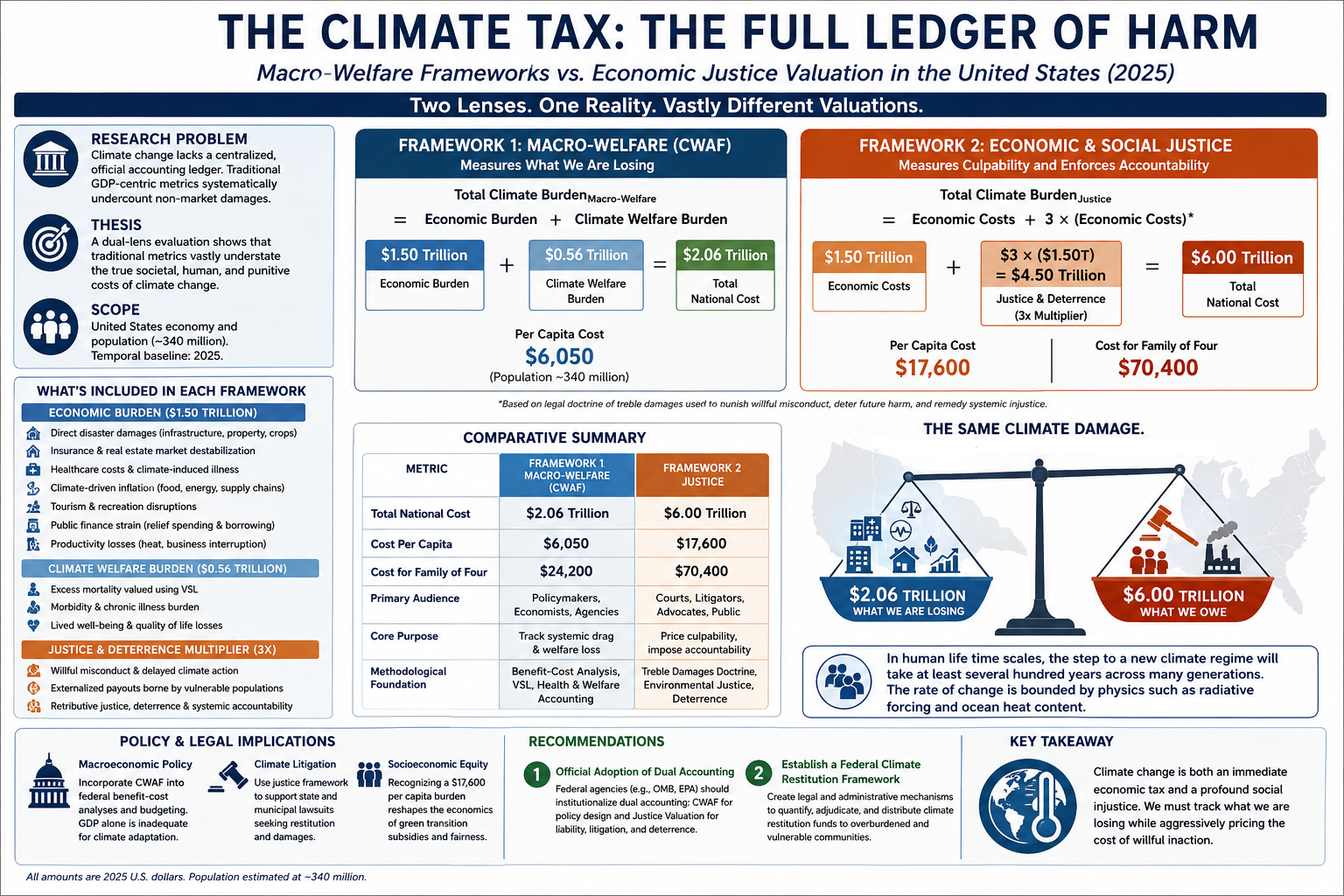
The two graphics accompanying this article illustrate the point. They were created from essentially the same prompt using two different AI systems. The Google version is estimated to have required roughly 25% fewer tokens, making it somewhat more computationally efficient, while the ChatGPT version produced a result I judged to have slightly greater marketing impact.
From an economic standpoint, the comparison is striking. Producing comparable illustrations through traditional methods could easily require hundreds of dollars in labor, software, revisions, and project management, along with the associated energy and material costs of conventional production. By contrast, the AI-generated graphics required only minutes to produce and incurred essentially no direct production cost beyond access to the AI platforms.
Although precise energy, water, and material consumption varies by hardware, data center design, and electricity source, my estimates suggest that using AI tools for this project reduced total resource consumption by well over 99% compared with creating equivalent graphics entirely through traditional manual workflows. In my own workflow, the estimated natural-resource cost was only a few cents per image.
This experience reinforces an important economic principle: productivity gains are often accompanied by reductions in resource intensity. When modern AI infrastructure is designed efficiently, it has the potential to reduce not only labor costs but also energy consumption, material use, water consumption, and overall environmental impact. Like any technology, AI should be evaluated based on measurable outcomes rather than assumptions. As the underlying infrastructure continues to improve, the environmental efficiency of these systems is likely to improve as well.
But, But, But… What About All the Other Costs and Environmental Impacts?
I understand your concerns—they’re important goals that I share. That’s why I’ve written this article explaining why I believe the benefits of modern AI infrastructure can outweigh the costs when it’s designed responsibly.
Ironically, many of the newest data center technologies can help advance the very objectives often listed. They’re becoming far more water-efficient through closed-loop cooling, more energy-efficient through advanced hardware and optical networking, and can reduce material demand by replacing large amounts of copper with fiber. AI is also accelerating the design of better batteries, more efficient renewable energy systems, smarter electrical grids, and improved land-use planning—all of which can help reduce environmental impacts over time.
From an economic perspective, I’ve found AI to be extraordinarily productive. One of our economic models projects that AI-driven automation could reduce the demand for human labor by as much as 90% over the next decade. Whether that estimate proves accurate or not, the broader trend points toward substantial productivity gains.
To me, that means the bigger societal question isn’t simply whether to build AI infrastructure. It’s how we prepare for an economy where productivity increasingly comes from intelligent systems. Issues like universal basic income, negative income taxes, wage subsidies, or other forms of national or global income support may become some of the most important policy discussions of the coming decades.
Technology itself isn’t inherently good or bad. The challenge is ensuring we deploy it in ways that improve both human well-being and environmental sustainability.
The original purpose of Solutions to the Fossil Fuel Economy and the Myths Accelerating Climate and Economic Collapse was to focus on practical solutions rather than assigning blame. Since its publication, however, many readers have interpreted that emphasis as minimizing the responsibility of fossil fuel companies. This addendum clarifies that both interpretations can be true simultaneously.
I began my career as an economist specializing in risk management before turning my attention to humanity’s largest systemic risk—climate change. My work spans economics, systems science, statistics, and climate physics. Together with physicist Sidd Mukherjee, I co-originated the Nonlinear Acceleration Hypothesis, a framework describing how interacting physical, ecological, health, and socioeconomic feedbacks can accelerate climate impacts beyond traditional linear projections.
My work has consistently argued that climate change is both a physical and an economic problem. It cannot be understood through atmospheric science alone, nor through economics alone. Rather, it emerges from the interaction of nonlinear Earth-system processes and human decision-making.
Shared Responsibility Does Not Eliminate Corporate Accountability
Fossil fuel consumption is fundamentally a supply-and-demand system. Producers cannot exist without consumers, and consumers cannot purchase what is not supplied. Responsibility therefore exists on multiple levels.
Recognizing consumer responsibility does not absolve fossil fuel companies of their own responsibilities.
Oil and gas companies have exercised enormous influence through lobbying, political advocacy, public relations campaigns, strategic communications, and efforts to delay or weaken climate policy. Those actions deserve careful scrutiny and, where appropriate, legal accountability.
At the same time, it is equally inaccurate to argue that consumers possess no agency whatsoever. While choices are often constrained by infrastructure, income, geography, and available technology, millions of individuals, businesses, and governments have successfully reduced fossil fuel dependence through efficiency improvements, electrification, renewable energy adoption, and changes in consumption patterns.
The issue is therefore not one of assigning exclusive blame to either producers or consumers. Climate change is the product of interacting economic incentives, political institutions, technological development, consumer behavior, and physical climate feedbacks.
Understanding that complexity is essential if society intends to solve the problem rather than merely redistribute blame.
Corporate Accountability
My work has also extensively examined legal and economic mechanisms for holding fossil fuel companies accountable, including:
climate litigation,
consumer protection law,
human rights frameworks,
carbon pricing and taxation,
restitution,
treble-damage recovery, and
broader climate liability frameworks.
Those topics are discussed in detail throughout the following papers, which complement the original economics article rather than contradict it.
The Fossil Fuel Industry
Oil and gas companies unquestionably bear significant responsibility for the climate crisis. Decades of internal research, lobbying, public relations campaigns, political influence, and efforts to delay emissions reductions have been extensively documented. Protecting market share and shareholder value frequently took precedence over communicating known climate risks or accelerating the transition to lower-carbon energy sources.
Those actions deserve public scrutiny and, where appropriate, legal accountability.
However, acknowledging corporate misconduct does not eliminate the role of consumer demand. Energy markets function through supply and demand. Producers extract, refine, and distribute fossil fuels because governments, businesses, and consumers continue to purchase them across transportation, electricity generation, manufacturing, agriculture, aviation, shipping, and residential heating.
This is not a moral judgment; it is an economic reality.
Consumers often operate within real constraints. Infrastructure, housing, public transportation, income, local utility policies, and technology availability all influence individual choices. Some households possess far greater flexibility than others. Nevertheless, constrained choice is not the same as no choice. Millions of households and businesses have reduced fossil fuel consumption through energy efficiency, electrification, renewable energy, improved building design, vehicle selection, and changes in consumption patterns. Each reduction weakens demand at the margin.
Likewise, governments influence both supply and demand through regulation, taxation, subsidies, infrastructure investments, and public procurement. Climate policy therefore operates across every level of society rather than through a single actor.
The climate crisis emerged from interacting physical, economic, technological, and political systems. Effective solutions require addressing each component simultaneously.
Existing Work on Corporate Accountability
Contrary to claims that emphasizing consumer responsibility somehow absolves fossil fuel producers, much of my work focuses specifically on legal and economic accountability for corporate misconduct.
The following papers examine those issues in detail.
Climate Change and Accountability
Climate Change and Accountability: Legal Challenges, Consumer Rights, and Human Rights in the Fight Against Fossil Fuels
This paper examines the legal foundations for climate litigation, including consumer fraud, public nuisance, deceptive marketing, human rights claims, restitution, and the application of legal principles similar to those successfully employed against the tobacco industry.
The Economics of Climate Change
Climate change is fundamentally different from most economic shocks.
Traditional recessions eventually recover. Financial crises stabilize. Commodity shortages resolve. Climate change does not naturally return to equilibrium within human timescales because excess greenhouse gases and accumulated ocean heat continue influencing the climate system for decades to centuries.
As University of Cape Town researcher Christopher Trisos observed:
“For people, other species, ecosystems, and the world we live in, we’ve entered the Age of Loss and Damage, but we’re just at the start.”
Likewise, following the record-breaking Northern Hemisphere summer of 2023, United Nations Secretary-General António Guterres warned:
“Climate breakdown has begun.”
These statements reflect a growing recognition that climate damages are no longer primarily future risks—they have become ongoing economic realities.
The Age of Loss and Damage
Climate economics must therefore evolve beyond traditional Integrated Assessment Models (IAMs), many of which assume smooth, gradual damage functions that underestimate systemic risk.
My work argues that climate damages arise from interacting nonlinear feedbacks operating simultaneously across physical, ecological, health, financial, insurance, agricultural, infrastructure, and geopolitical systems.
Understanding those interactions requires integrating:
economics,
systems science,
statistics,
atmospheric physics,
ecology,
public health, and
risk management.
The resulting framework is consistent with the Nonlinear Acceleration Hypothesis, which recognizes that climate impacts increasingly reinforce one another through cascading feedback loops rather than simple linear cause-and-effect relationships.
Accounting for Climate Damages
One objective of climate economics is not merely estimating annual losses, but accounting for the full societal burden imposed by delayed mitigation and continued emissions.
Quantifying the Climate Tax
Quantifying the Climate Tax: The Full Ledger of Harm
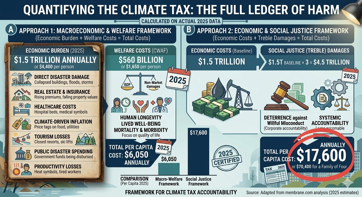
This paper estimates the annual economic burden currently imposed by climate change on American households.
The analysis concludes that the direct annual climate burden already approaches $6,000 per person, while the broader long-term burden—including infrastructure degradation, ecosystem loss, health impacts, insurance instability, productivity losses, and deferred damages imposed on future generations—is substantially larger.
Climate change is therefore functioning as an invisible tax already embedded throughout the economy.
The Legal Foundation for Treble Damages
American law has long recognized that ordinary compensation is insufficient when misconduct is deliberate, deceptive, or socially destructive.
Treble damages appear throughout U.S. law, including:
Sherman Act antitrust litigation,
RICO actions,
False Claims Act enforcement, and
numerous state consumer protection statutes.
Their purpose extends beyond compensation. They deter future misconduct while recognizing that direct damages frequently underestimate total societal harm.
A comparable framework may be appropriate when evaluating climate-related damages if plaintiffs establish that institutions knowingly delayed mitigation while externalizing foreseeable risks onto the public.
Justice, Restitution, and Climate Liability
Applying a justice framework to climate economics raises three related questions:
Did organizations knowingly externalize foreseeable climate damages?
Have those damages fallen disproportionately upon vulnerable populations and future generations?
Should legal remedies reflect deterrence as well as compensation?
These questions extend beyond economics into ethics, law, and public policy, but they are increasingly becoming central to climate litigation worldwide.
The Cost of Inaction
The companion paper,
The Full Economic Burden: An Ensemble-Based Probabilistic Framework
develops an ensemble-based probabilistic framework for estimating the long-term economic consequences of accelerating climate change.
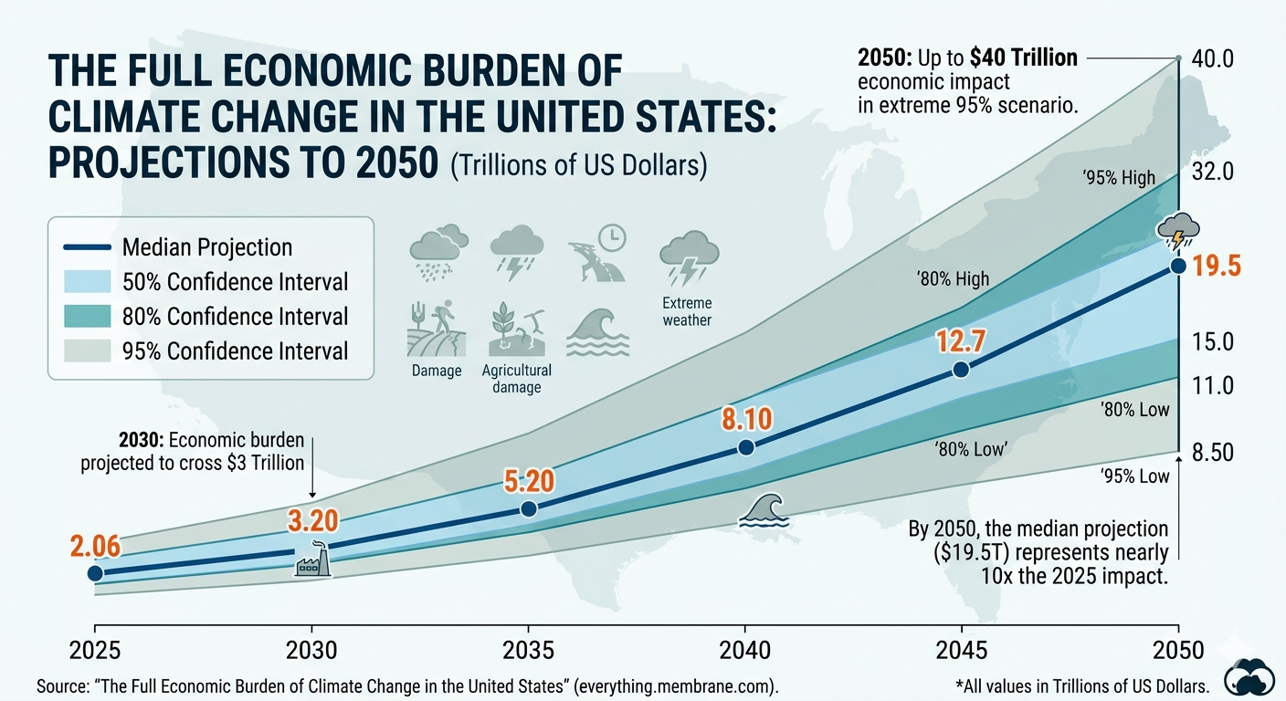
Under the median ensemble projection, annual U.S. climate-related economic losses increase nearly tenfold, rising from approximately $2.1 trillion in 2025 to $19.5 trillion by 2050 (constant 2025 dollars).
Rather than projecting a steady increase in damages, the analysis demonstrates how interacting physical, ecological, health, financial, and socioeconomic feedbacks can transform climate change into an accelerating systemic economic burden.
Under the median ensemble scenario, cumulative U.S. climate-related losses between 2025 and 2050 approach $200 trillion (constant 2025 dollars).
These projections illustrate a central conclusion of the Nonlinear Acceleration Hypothesis: delayed responses, thermal inertia, interacting feedbacks, and tipping cascades can produce economic impacts that grow substantially faster than traditional linear or quadratic damage models anticipate.
Conclusion
Climate responsibility should never be framed as an either-or proposition.
Corporations that knowingly delayed climate action should be held accountable through transparent governance, appropriate regulation, and where justified, legal remedies.
Governments bear responsibility for designing policies that correctly price externalities, accelerate innovation, and remove barriers to decarbonization.
Businesses bear responsibility for reducing emissions throughout their operations and supply chains.
Consumers also retain agency through the choices they make within the constraints they face.
Climate change emerged from the interaction of all of these systems. Lasting solutions will require accountability and action across all of them.
Transpiration is the biological process by which plants move water from the soil through their roots and vascular system and release it into the atmosphere as water vapor. This release occurs through microscopic pores on leaves called stomata, which also regulate carbon dioxide intake for photosynthesis.
In simple terms, transpiration is the plant equivalent of sweating:
Plants absorb water from soil
Transport it upward through xylem tissue
Release it as vapor through leaf stomata
Although it is a natural biological function, transpiration is also a major component of Earth’s water cycle and climate system.
Why Transpiration Matters
1. Nutrient transport
Water pulled upward by transpiration carries essential minerals from soil into leaves and stems, enabling plant growth and metabolism.
2. Natural cooling system
When water evaporates from leaves, it absorbs energy as latent heat, cooling both the plant and surrounding air. Large forests can significantly reduce local temperatures through this process.
3. Rainfall and atmospheric moisture recycling
Ecosystems such as tropical rainforests return enormous amounts of water vapor to the atmosphere. This moisture contributes to cloud formation and rainfall, often sustaining the very ecosystems that produce it.
How Transpiration Works (Step-by-Step)
Absorption: Roots draw water and dissolved nutrients from soil.
Transport: Water moves upward through xylem under tension.
Regulation: Stomata open and close to balance CO₂ intake and water loss.
Evaporation: Water exits leaves as vapor, entering the atmosphere.
Transpiration and Climate Change: A Shifting System
Transpiration is highly sensitive to temperature, humidity, and atmospheric composition. As the climate warms, these conditions are changing rapidly—and not always in the same direction.
The Clausius–Clapeyron Relationship: Why Warm Air Changes Everything
A key physical principle in climate science is the Clausius–Clapeyron relationship, which states that warmer air can hold more water vapor.
In practical terms:
For every ~1°C of warming, the atmosphere can hold about 7% more moisture
This increases the atmosphere’s evaporative demand
This relationship drives a critical climate variable: vapor pressure deficit (VPD)—the difference between how much moisture air can hold and how much it actually contains.
As temperatures rise:
VPD increases
The atmosphere draws more moisture from soils and plants
Evaporation and transpiration rates accelerate
This creates a powerful “drying force” on vegetation and soils.
Why Transpiration Can Increase—and Then Collapse
Climate change creates a competing set of forces:
1. Atmospheric acceleration (increased water loss)
Higher temperatures increase evaporation demand
Higher VPD pulls more moisture from leaves and soil
Early warming stages often increase transpiration rates
2. Plant regulation (defensive shutdown)
Plants respond to water stress by closing stomata:
Reduces water loss
But also reduces CO₂ uptake
Weakens photosynthesis and ecosystem productivity
At large scales, this can reduce regional moisture recycling.
Loss of Biosphere Cooling
Transpiration is also a major cooling mechanism for Earth’s surface.
When water evaporates from leaves:
Energy is absorbed as latent heat
Air temperatures are reduced locally
But when plants close stomata or soil moisture declines:
Latent cooling weakens
More solar energy becomes sensible heat
Local temperatures rise further
This can intensify heat extremes during heat waves.
Forest Moisture Recycling and System Stability
Large forests—especially tropical rainforests—depend on internal moisture recycling:
Trees transpire water vapor
Vapor forms clouds
Clouds produce rainfall
Rain sustains the forest
If transpiration declines:
Rainfall decreases
Dry seasons lengthen
Vegetation stress increases
This creates a feedback loop: less transpiration → less rainfall → more drought → further forest loss
Agricultural Amplification: Corn Sweat, Humidity, and Human Heat Risk
Large agricultural systems can significantly alter local atmospheric conditions through transpiration. One of the most well-known examples is “corn sweat.”
A mature cornfield during peak summer heat can release thousands of gallons of water per acre per day into the atmosphere. This moisture increases local humidity and can meaningfully alter how heat is experienced by humans.
From Heat to Danger: Why Humidity Matters
Human cooling depends on evaporation of sweat. When humidity is high:
Sweat evaporates more slowly
Body heat is trapped
Core temperature rises faster
This is where wet-bulb temperature becomes critical.
Wet-bulb temperature combines:
Air temperature
Humidity
It represents the physical limit of human heat tolerance because it determines whether sweat can still cool the body.
Corn Sweat and Rising Wet-Bulb Stress
Corn transpiration adds moisture to air masses already warmed by climate change. When combined with rising temperatures:
Atmospheric moisture increases
Humidity rises sharply
Wet-bulb temperature increases faster than air temperature alone
This combination can push conditions closer to dangerous physiological thresholds even when air temperature appears only moderately high.
Expanding Heat Danger into New Regions
Historically, dangerous humid heat in the United States was concentrated in:
The Gulf Coast
Parts of the Southeast
However, as climate patterns shift:
Heat and humidity extremes are moving northward and inland
The Midwest increasingly experiences high humidity heat events
Regions like Iowa, Illinois, Indiana, Missouri, and Ohio are seeing more frequent dangerous combinations of heat and moisture
These are areas that historically did not experience prolonged conditions where outdoor physical activity becomes unsafe due to humidity-driven heat stress.
Heat Alert Days and Human Exposure
A growing concern is the increase in heat alert days—days when outdoor exertion becomes unsafe or strongly discouraged.
Contributing factors include:
More frequent heat waves
Higher humidity levels
Reduced nighttime cooling
Impacts include:
Increased heat exhaustion and heat stroke risk
Reduced safe working hours for outdoor labor
Greater strain on agriculture, construction, and public health systems
Importantly, risk is no longer defined by temperature alone. Humidity-driven heat stress is becoming a dominant factor.
Soil: The Hidden Climate Regulator
Soil plays a central role in regulating transpiration and climate stability.
Healthy soil:
Stores water for plants
Supports microbial ecosystems
Helps regulate carbon cycling
Degraded soil:
Loses moisture retention capacity
Reduces plant resilience
Releases stored carbon
When soils degrade into desertified states, transpiration systems weaken, reducing both cooling and rainfall feedbacks.
Conclusion
Transpiration is not just a plant process—it is a core component of Earth’s climate system. It links soil, vegetation, and atmosphere through continuous water and energy exchange.
Under climate change, transpiration is being reshaped by:
The Clausius–Clapeyron-driven increase in atmospheric moisture capacity
Rising vapor pressure deficits
Plant stomatal responses to heat and CO₂
Large-scale ecosystem stress and land-use change
These shifts affect not only ecosystems but also human health. Agricultural moisture release, such as corn sweat, interacts with warming temperatures to increase humidity and elevate wet-bulb temperatures—expanding regions where outdoor exertion becomes dangerous.
The result is a climate system in which biological, atmospheric, and human factors are increasingly interconnected—and increasingly strained under continued warming.
During the 1980s, I worked primarily as an economist specializing in risk management. By the early 1990s, however, it had become clear that the greatest systemic risk facing civilization was not financial—it was climate change.
Working with physicist Sidd Mukherjee, we began developing what we called the Nonlinear Acceleration Hypothesis: the idea that climate change would not progress as a slow, linear process, but instead would accelerate as reinforcing Earth-system feedbacks became increasingly dominant.
Over the past three decades, an expanding body of observational evidence has increasingly supported this perspective. Today, nonlinear climate dynamics, positive feedbacks, tipping points, and cascading Earth-system interactions have become central concepts within modern climate science and climate-risk research.
From Linear Assumptions to Nonlinear Reality
By 1995, I had become convinced that many climate indicators were evolving exponentially rather than linearly. Sidd agreed the hypothesis was plausible but argued that a much longer observational record would be necessary before drawing firm conclusions.
At the time, most climate projections implicitly assumed relatively gradual warming. While serious, climate change was generally viewed as unfolding over centuries, leaving substantial time for adaptation and mitigation.
Yet observational evidence already suggested something different. Looking beyond annual variability, many climate indicators appeared to be accelerating.
By 2004, sufficient observations had accumulated to demonstrate nonlinear behavior across multiple components of the Earth system. Greenland Ice Sheet dynamics, in particular, were no longer consistent with simple equilibrium assumptions. Ocean heat uptake, ice-sheet mass loss, atmospheric moisture, and extreme precipitation all exhibited increasing rates of change.
A striking pattern emerged.
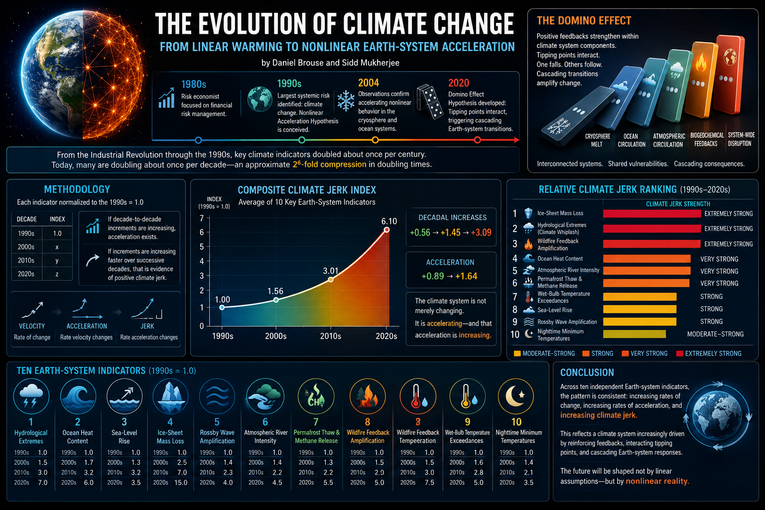
From the Industrial Revolution through approximately the 1990s, many leading indicators of climate change appeared to double on timescales approaching one century.
Today, many of those same indicators are doubling on timescales measured in roughly one decade.
This represents an approximate 2⁶-fold compression of doubling times over successive decades—a remarkable acceleration in the pace of climate change.
Rather than simply warming faster, the Earth system appears to be evolving into an increasingly nonlinear state in which the rate of change itself continues to accelerate.
If sustained, this may represent one of the most abrupt large-scale climate transitions in Earth’s geological history.
The Domino Effect
By 2020, our work expanded into what we termed the Domino Effect Hypothesis.
Many components of the climate system contain internal positive feedback mechanisms. As these feedbacks strengthen, the climate system becomes progressively less dependent upon external forcing because it increasingly reinforces its own evolution.
These critical threshold transitions are commonly known as climate tipping points.
Unlike gradual warming, tipping points exhibit nonlinear behavior in which relatively small additional forcing can produce disproportionately large—and potentially irreversible—changes.
Even more importantly, tipping points rarely occur in isolation.
The atmosphere, oceans, cryosphere, biosphere, and carbon cycle are tightly interconnected. Destabilization within one subsystem can reduce the stability of others, producing a sequence of interacting transitions throughout the Earth system.
This cascading behavior—often referred to as tipping cascades—forms the basis of the Domino Effect.
Since its proposal, extensive observational evidence has demonstrated that interacting climate feedbacks are a defining feature of modern climate dynamics and now occupy a central position within contemporary climate-risk literature.
Methodology
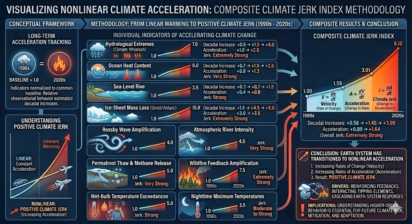
To illustrate long-term changes in climate acceleration, each indicator was normalized to a common baseline:
1990s = 1.0
Relative observational behavior was then estimated for each subsequent decade.
If the decade-to-decade increases become progressively larger, the indicator exhibits positive acceleration.
If the acceleration itself continues increasing over time, this represents positive climate jerk—the rate at which acceleration is increasing.
In physics:
Velocity describes the rate of change.
Acceleration describes the rate at which velocity changes.
Jerk describes the rate at which acceleration changes.
Applied to climate science, positive climate jerk indicates that Earth’s climate is not simply changing faster—it is accelerating faster over time.
1. Hydrological Extremes and Climate Whiplash
Decade
Index
1990s
1.0
2000s
1.5
2010s
3.0
2020s
7.0
Decadal increase: +0.5 → +1.5 → +4.0
Acceleration: +1.0 → +2.5
Climate Jerk:Extremely Strong
2. Ocean Heat Content
Decade
Index
1990s
1.0
2000s
1.7
2010s
3.2
2020s
6.0
Decadal increase: +0.7 → +1.5 → +2.8
Acceleration: +0.8 → +1.3
Climate Jerk:Very Strong
3. Sea-Level Rise
Decade
Index
1990s
1.0
2000s
1.3
2010s
2.0
2020s
3.5
Decadal increase: +0.3 → +0.7 → +1.5
Acceleration: +0.4 → +0.8
Climate Jerk:Strong
4. Ice-Sheet Mass Loss
(Greenland and Antarctica Combined)
Decade
Index
1990s
1.0
2000s
2.5
2010s
7.0
2020s
15.0
Decadal increase: +1.5 → +4.5 → +8.0
Acceleration: +3.0 → +3.5
Climate Jerk:Extremely Strong
5. Rossby Wave Amplification
Decade
Index
1990s
1.0
2000s
1.4
2010s
2.3
2020s
4.0
Climate Jerk:Strong
6. Atmospheric River Intensity
Decade
Index
1990s
1.0
2000s
1.3
2010s
2.2
2020s
4.5
Climate Jerk:Very Strong
7. Permafrost Thaw and Methane Release
Decade
Index
1990s
1.0
2000s
1.4
2010s
2.5
2020s
5.0
Climate Jerk:Very Strong
8. Wildfire Feedback Amplification
Decade
Index
1990s
1.0
2000s
1.5
2010s
3.0
2020s
7.5
Climate Jerk:Extremely Strong
9. Wet-Bulb Temperature Exceedances
Decade
Index
1990s
1.0
2000s
1.6
2010s
2.8
2020s
5.0
Climate Jerk:Strong
10. Nighttime Minimum Temperatures
Decade
Index
1990s
1.0
2000s
1.4
2010s
2.1
2020s
3.5
Climate Jerk:Moderate to Strong
Composite Climate Jerk Index
A simple average of the ten normalized indicators produces the following composite behavior:
Decade
Composite Index
1990s
1.00
2000s
1.56
2010s
3.01
2020s
6.10
Decadal increases
+0.56 → +1.45 → +3.09
Acceleration
+0.89 → +1.64
Conclusion
Viewed collectively, these observational indicators suggest that the Earth’s climate system has undergone a profound transition since the late twentieth century. The evidence indicates not only increasing rates of change, but increasing rates of acceleration—a phenomenon that may be described as positive climate jerk.
This behavior is consistent with a climate system increasingly influenced by reinforcing feedbacks, interacting tipping elements, and cascading Earth-system responses.
Whether evaluated through ice-sheet dynamics, ocean heat uptake, hydrological extremes, atmospheric circulation, wildfire amplification, or permafrost thaw, the emerging pattern is remarkably consistent: the climate system is not merely changing—it is accelerating, and that acceleration itself continues to increase.
Understanding this higher-order behavior may prove essential for accurately assessing future climate risk and for developing mitigation and adaptation strategies that account for the nonlinear dynamics of the Earth system.
Climate Tipping Points and Cascading Feedbacks: Assessing the Current State of Earth’s Critical Climate Systems (2026 Review)
Daniel Brouse and Sidd Mukherjee
June 2026
Abstract
Climate change is no longer characterized solely by gradual increases in global temperature. A growing body of observational evidence demonstrates that multiple components of the Earth system are approaching—or in several cases have entered—states of self-reinforcing change driven by positive climate feedbacks. These nonlinear transitions, known as climate tipping points, increase the likelihood that future warming will proceed more rapidly than would be expected from anthropogenic greenhouse gas emissions alone.
This review synthesizes observational evidence through 2026 regarding the status of the Earth’s principal climate tipping elements, including the Greenland and West Antarctic Ice Sheets, the Atlantic Meridional Overturning Circulation (AMOC), Arctic permafrost, coral reefs, mountain glaciers, boreal forests, and the Amazon rainforest. Rather than functioning independently, these systems interact through atmospheric, oceanic, cryospheric, and carbon-cycle feedbacks that may produce cascading or “domino” effects across the Earth system.
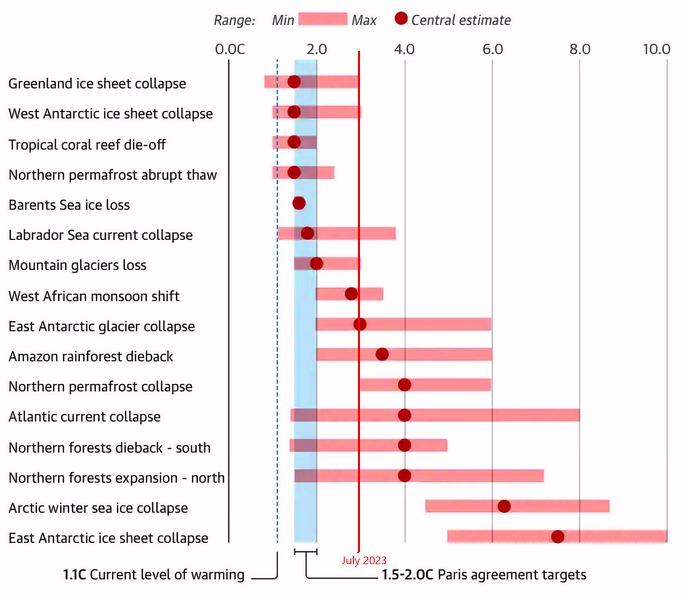
Recent observations—including record ocean heat content, accelerating sea-level rise, unprecedented marine heatwaves, widespread coral bleaching, Arctic amplification, increasing atmospheric moisture, and rapid changes in hydrologic extremes—indicate that Earth is entering a period in which nonlinear feedbacks are becoming increasingly important drivers of climate evolution. Although considerable uncertainty remains regarding the precise thresholds and timing of individual tipping elements, evidence suggests that the probability of interacting tipping cascades increases substantially as global warming approaches and exceeds 1.5–2.0°C above pre-industrial temperatures.
1. Introduction
For decades climate change was commonly portrayed as a gradual, approximately linear response to increasing greenhouse gas concentrations. While this approximation remains useful for estimating long-term average warming, it does not fully describe how complex Earth systems behave near critical thresholds.
Many components of the climate system contain internal positive feedback mechanisms. Once these mechanisms become sufficiently strong, additional external forcing becomes progressively less important as the system begins reinforcing its own evolution.
These threshold transitions are known as climate tipping points.
Unlike gradual climate change, tipping points involve nonlinear behavior in which relatively small additional changes in forcing can trigger disproportionately large and potentially long-lasting responses.
Perhaps more importantly, tipping points do not occur in isolation. They interact through atmospheric circulation, ocean circulation, carbon cycling, and cryospheric processes. The destabilization of one system can reduce the stability of another, producing cascading transitions across the Earth system—a phenomenon often referred to as tipping cascades or the Domino Effect.
2. Climate Feedbacks: The Engine of Acceleration
Every climate tipping point is driven by positive feedback loops.
Examples include:
Ice-albedo feedback
Water-vapor amplification
Permafrost carbon release
Forest-fire carbon emissions
Vegetation dieback
Ocean heat uptake
Cloud feedbacks
Positive feedbacks increase warming.
Negative feedbacks partially offset warming.
As temperatures rise, positive feedbacks become increasingly dominant within several major Earth systems.
The practical consequence is acceleration.
Instead of climate change progressing at a nearly constant rate, the rate of change itself increases over time.
3. Current Status of Major Climate Tipping Elements
Warm-Water Coral Reefs
Current evidence indicates that tropical coral reefs have become the first major global ecosystem to exhibit widespread tipping behavior.
Mass bleaching events have occurred repeatedly since 2016 and culminated in an unprecedented global bleaching episode during 2023–2025.
Although individual reefs may recover, many reef systems have shifted toward persistent ecological degradation.
Current assessment: Actively tipping
Mountain Glaciers
Mountain glaciers are retreating in nearly every mountain range worldwide.
Many glaciers have already lost sufficient mass that complete disappearance has become unavoidable regardless of future emissions reductions.
Consequences include:
declining freshwater supplies
increased hazards from glacial lakes
long-term contributions to sea-level rise
Current assessment: Long-term loss committed in many regions
Greenland Ice Sheet
The Greenland Ice Sheet continues to lose mass at an accelerating rate.
Surface melting, increased rainfall, darker ice surfaces, and elevation feedbacks are reinforcing one another.
Current evidence suggests that portions of Greenland may already be committed to long-term ice loss under present warming levels, although complete deglaciation would require centuries to millennia.
Current assessment: Actively destabilizing
West Antarctic Ice Sheet
Marine ice-sheet instability is progressing in several sectors of West Antarctica, particularly near Thwaites and Pine Island glaciers.
Ocean warming beneath floating ice shelves continues to reduce buttressing, increasing ice discharge into the Southern Ocean.
Although complete collapse remains uncertain in timing, several marine basins now appear vulnerable to irreversible retreat.
Current assessment: High confidence of ongoing destabilization
Arctic Permafrost
Abrupt thaw, thermokarst formation, methane emissions, and increasing wildfire activity are altering large portions of Arctic permafrost.
These changes reduce one of Earth’s largest terrestrial carbon reservoirs while increasing greenhouse gas emissions.
The AMOC has weakened substantially over the past century.
Freshwater from Greenland melt, increased precipitation, and Arctic warming continue to reduce North Atlantic surface-water density.
While the timing of any future collapse remains uncertain, observations indicate that resilience has declined.
Current assessment: Weakening with elevated tipping risk
Amazon Rainforest
The Amazon faces simultaneous stress from warming, drought, wildfire, and deforestation.
Southern portions of the basin have already shifted from net carbon sink toward seasonal carbon source.
Large-scale forest dieback would reduce rainfall recycling and amplify regional drying.
Current assessment: Fragmenting under combined climate and land-use pressures
Boreal Forests
Increasing wildfire activity, insect outbreaks, and drought are transforming boreal ecosystems across Canada, Alaska, and Siberia.
These forests are migrating northward while losing biomass across their southern margins.
Current assessment: Increasing ecological stress
4. Interacting Climate Cascades
The greatest concern is not any single tipping point.
It is their interaction.
The Greenland Ice Sheet provides a clear example.
Accelerated melting introduces freshwater into the North Atlantic → Freshwater weakens deep-water formation → AMOC slows → Ocean heat redistributes toward the Southern Hemisphere → Additional heat reaches West Antarctica → Ice-sheet instability increases → Sea-level rise accelerates
Meanwhile:
AMOC weakening alters atmospheric circulation → South American rainfall decreases → Amazon drought intensifies → Forest dieback increases → Carbon emissions rise → Global warming accelerates
This sequence illustrates how apparently separate climate systems become mechanically coupled.
5. Emerging Indicators of Nonlinear Climate Change (2025–2026)
Several observational indicators suggest acceleration is occurring across multiple components of the climate system.
Among the strongest indicators are:
Record global ocean heat content
Increasing Earth energy imbalance
Accelerating marine heatwaves
Increasing atmospheric moisture
Stronger atmospheric rivers
More persistent Rossby-wave blocking
Arctic amplification
Accelerating sea-level rise
Longer wildfire seasons
More rapid permafrost thaw
Increasing nighttime temperatures
Greater frequency of compound drought–flood events
Individually these indicators do not prove tipping cascades.
Collectively they demonstrate increasing instability throughout the climate system.
6. The Domino Effect
Climate tipping points should not be viewed as isolated thresholds.
They function as an interconnected network.
Positive feedbacks reinforce warming.
Warming destabilizes tipping elements.
Destabilized tipping elements activate additional feedbacks.
Those additional feedbacks increase warming further.
The process repeats.
This cascading behavior compresses climate timescales.
Processes once expected over centuries may increasingly unfold over decades in vulnerable regions.
Although considerable uncertainty remains regarding the exact timing of future transitions, the probability of interacting tipping cascades increases as warming continues.
The Domino Effect: An example of an interacting Earth-system cascade
Polar amplification → reduced equator-to-pole temperature gradient → weakened thermal contrast that influences large-scale atmospheric circulation → accelerated Arctic and Greenland ice loss → increased freshwater discharge into the North Atlantic, reducing surface-water salinity and density → weakening of deep-water formation and increasing risk of Atlantic Meridional Overturning Circulation (AMOC) slowdown → reorganization of North Atlantic pressure patterns and storm tracks → greater jet-stream waviness, slower progression, and amplified Rossby-wave behavior → more persistent blocking patterns, omega blocks, and meridional flow → longer-lasting atmospheric rivers, heat domes, drought–flood whiplash, and other hydroclimatic extremes → increasing stress on agriculture, infrastructure, ecosystems, water resources, and public health → continued land-ice loss and groundwater redistribution that alter Earth’s mass distribution → climate-driven mass redistribution sufficient to measurably change Earth’s moment of inertia, contributing to small changes in Earth’s rotation and the length of day.
7. Scientific Uncertainty
Significant uncertainties remain.
Researchers continue to debate:
precise temperature thresholds
rates of future ice-sheet response
methane release from permafrost
resilience of tropical forests
future behavior of the AMOC
interactions among multiple tipping elements
These uncertainties should not be interpreted as evidence that tipping points are absent.
Rather, they reflect the complexity of coupled nonlinear Earth systems.
The direction of change is well established.
The exact timing remains uncertain.
8. Conclusions
Observations through 2026 indicate that Earth is entering a period in which nonlinear climate feedbacks are becoming increasingly important.
Several climate systems—including warm-water coral reefs, mountain glaciers, portions of the Greenland Ice Sheet, Arctic permafrost, and sectors of the West Antarctic Ice Sheet—are exhibiting sustained changes consistent with increasing instability.
Other systems, including the AMOC and Amazon rainforest, remain highly vulnerable as global temperatures continue to rise.
The principal scientific challenge is no longer identifying individual tipping points. It is understanding how they interact.
The emerging evidence suggests that the Earth’s major climate systems function less like isolated components than as an interconnected network linked by feedback loops, energy flows, and atmospheric and oceanic circulation.
Whether future climate change remains relatively manageable or evolves into a series of cascading transitions will depend largely on the magnitude and duration of future warming.
While some long-term changes may already be committed because of internal feedbacks, rapid reductions in greenhouse gas emissions can still substantially reduce the likelihood, speed, and severity of additional tipping cascades.
The coming decades will determine not only how much the planet warms, but whether multiple Earth-system tipping elements remain largely independent or become synchronized into a self-reinforcing global transition.
Tipped Tipping Points, Feedback Loops, and the Domino Effect
Feedback Loops → Tipping Points → Acceleration → Domino Effect Feedback loops amplify climate change and can push interconnected Earth systems past critical tipping points. As tipping points are crossed, they can trigger additional feedback loops and destabilize other climate systems. This cascading “Domino Effect” compresses timescales, accelerates change, and increases the risk of rapid, nonlinear climate transformations.
By Daniel Brouse and Sidd Mukherjee September 29, 2023, and November 12, 2023
Identifying and understanding these tipping points is crucial for climate science and policymaking. Crossing multiple tipping points could lead to a domino effect, resulting in a much more rapid and severe climate change than currently projected.
Push a glass toward the edge of a table and eventually it will fall off on its own. No matter how slowly or meticulously you push… no matter how you weight or fill the glass, it will reach a tipping point and fall off before being pushed completely off the table. No matter whether you believe the glass is half-empty or half-full, when the tipping point is reached it will plummet out-of-control to its end. This is science not fate, faith, nor belief. Human induced climate change has resulted in environmental tipping points being breached.
Tipping points, when crossed, trigger self-sustaining feedback loops that are no longer dependent on human activity. Similar to when a domino topples over hitting two more dominoes that in turn fall hitting more dominoes. Thus, the name The Domino Effect. In literature, this is usually called:
cascading tipping points
tipping cascades
coupled nonlinear thresholds
It can also be visualized as The Snowball Effect. A tipping point is like a snowball rolling down a hill growing in mass and velocity (momentum). When a tipping point is crossed, it results in cumulative and reinforced global warming.
A look at seven of the nine tipping points crossed that show the proverbial snowball is already rolling. The first dominoes have fallen and will continue to knock down more tiles with each escalating step.
Mountain Glacier Loss
Greenland Ice Sheet Collapse
Antarctic Ice Sheet Collapse
Collapse of AMOC (Atlantic Meridional Overturning Circulation)
Amazon Rainforest Dieback
Coral Reef Die-Off
Northern Permafrost Collapse
Crossing even a single tipping point is alarming. For instance, crossing the tipping point for ‘mountain glacier loss‘ has immediate consequences: millions of people in Europe will be impacted by the lack of fresh water. Billions of people that live along coasts will be impacted by the saline infiltration and eventually by the submerging of their property. In September of 2022, UNESCO reported accelerated melting of glaciers in World Heritage sites, with glaciers in a third of sites set to disappear by 2050. In September of 2023, the GLAMOS glacier monitoring center found 10% of Swiss glaciers had disappeared in the last 2 years. They do not expect any Swiss glaciers will be left by 2050 no matter what actions are taken. If extreme measures are taken, they anticipate we may be able to save some polar glaciers.
This in and of itself should be alarming; however, it gets worse. Tipping points are parts of feedback loop systems. The ice-albedo feedback loop is an expression of the ability of surfaces to reflect sunlight (heat from the sun). Any loss of ice over a darker surface means the surface will absorb more heat and reflect less heat. This process makes the Earth warmer causing more loss of ice, which in turn causes more warming of the Earth. So, yes, the mountain ice tipping point is quite alarming for both its immediate impact as well as its self-sustaining growth to global warming; but wait, it gets more alarming. The increasing temperatures due to crossing a tipping point cause other tipping points to be toppled (The Domino Effect).
Update on Interactions and Feedbacks: An example of this is the converging collapse of the AMOC and the jet streams. This acceleration is driven by non-linear system failures across the AMOC, jet streams, and hydrological cycles — dynamics that traditional climate models have consistently underestimated. These shifts are not theoretical predictions for the distant future; they are being measured in real time right now.
By the Autumn of 2023, it had become evident the West Antarctic and Greenland ice sheets will completely melt. The process is irreversible and inevitable. The rain intensity is increasing faster today than ever known. The cool water from the melting ice at the poles is being drawn toward the center of the Earth and getting warmed to record high temperatures. The warm, moist air is circulating and moving over land. These changes in climate systems will cause other areas to experience unprecedented drought. We expect sea level rise will total about 270 feet over the next several millennia. It is episodic, and in the fast bits it can go up 3 feet every twenty years for five hundred years. The melting Arctic and Antarctic have multiple feedback loops including: enhanced oceanic heating and ice-albedo, Planck feedback, lapse-rate feedback, and cloud feedback.
The tipping point for the collapse of AMOC (Atlantic Meridional Overturning Circulation) was thought to be centuries away, at the earliest. In July of 2023, the study Warning of a forthcoming collapse of the Atlantic meridional overturning circulation was published in the journal Nature Communications. “Here we provide statistical significance and data-driven estimators for the time of tipping. We estimate a collapse of the AMOC to occur around mid-century (2025-2095) under the current scenario of future emissions.” The collapse is likely to cause faster sea level rise on the east coast of the US, more severe storms in Europe, and increasing drought in the Sahel in Africa. “From the study of past climate, we know changes in the AMOC have been some of the most abrupt and impactful events in the history of climate,” said Prof. Stefan Rahmstorf, at the Potsdam Institute for Climate Impact Research in Germany and world leading oceanographer. During the last Ice Age, winter temperatures changed by up to 10C within three years in some places. “We are dealing with a system that in some aspects is highly non-linear, so fiddling with it is very dangerous, because you may well trigger some surprises,” he said. “I wish I knew where this critical tipping point is, but that is unfortunately just what we don’t know. We should avoid disrupting the AMOC at all costs. It is one more reason why we should stop global warming as soon as possible.” A feedback loop created by the AMOC tipping point would cause a disruption of weather systems and circulation. The result would be the loss of naturally occurring carbon sinks. One scenario is desertification of the Amazon rainforest. In 2023, the Amazon River and the Rio Negro set record low levels.
The tipping point / feedback loop problem is very complex (chaos theory) and exponentially alarming. Yet another tipping point appears to have been triggered before 2024 — Amazon Rainforest Dieback. The Amazon is often referred to as ‘the lungs of our planet.’ Not only does the Amazon suck in huge quantities of CO2 and breath out O2, but the Amazon soils also store huge amounts of CO2. The desertification of the Amazon would result in a release of the carbon as the soils disappeared.
1) part of July was spent at record temperatures +3C 2) the collapse of the Amazon rainforest is likely to happen between +2 – 4C. The collapse of the Amazon is expected to occur because of changing weather patterns and circulation that result in drought. 3) Brazil set up a task force for “unprecedented drought in the Amazon”
Low river levels and hotter waters have killed masses of fish seen floating on river surfaces, contaminating the drinking water, Environment Minister Marina Silva said. “We have a very worrying situation. This record drought has disrupted river transport routes (dropping 30 cm / day) threatening food and water shortages, and a large fish mortality is already beginning.” This was the effect of a periodic El Nino mixing with changes in weather patterns brought by global warming. “We are seeing a collision of two phenomena, one natural which is El Nino and the other a phenomenon produced by humans, which is the change in the Earth’s temperature.” Worsened by climate change, this combination has caused drought not seen before in the Amazon and “is incomparably stronger and could happen more frequently.”
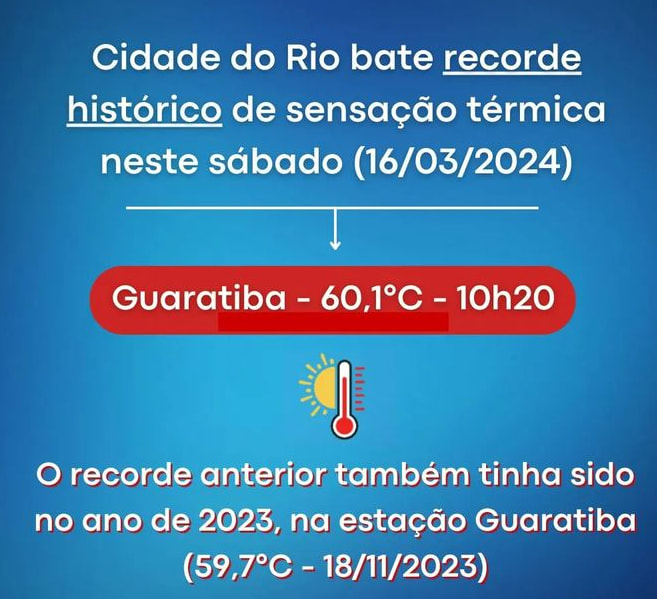
The average temperature for Brazil had been above the historical average from July through October of 2023. Rio de Janeiro recorded 42.5C on November 12, 2023 (a record for November) and high humidity on the 14th meant that it felt like 58.5C, municipal authorities said. Deadly humid heat is the greatest short term climate change risk to human health. On November 17, “a young Brazilian fan of US singer Taylor Swift died in Rio de Janeiro after falling ill inside the sweltering stadium where the superstar’s concert was held, amid a record-breaking heatwave across large swathes of Brazil,” as reported by ABC. “The show took place on the same day that Rio recorded its highest-ever heat index reading, which combines temperature and humidity, at 59.3 degrees Celsius (139 degrees Fahrenheit).”
Brazil’s Pantanal wetlands are famous for their paradise of biodiversity. There were 2,387 fires in the Pantanal in the first 13 days of November 2023, an increase of more than 1,000 percent from the entire month of November last year, according to satellite monitoring by Brazilian space research agency INPE. “The situation is completely out of control. And between the heatwave and the wind, it’s only going to get worse,” says biologist Gustavo Figueiroa, head of the environmental group SOS Pantanal.
What do you know about the Rio Negro as it relates to climate change and carbon sinks? The Rio Negro gets its name from its color. The black water is caused by highly acidic and carbon rich water. One scientist that lives on the river called it similar to Coca-cola. In 2023, the Rio Negro recorded record low levels.
Most of the carbon discharged into the water helps the carbon to eventually sink in the ocean as a literal carbon sink. The lack of rain and drought conditions result in more vegetation dying and contribute to a feedback loop — more plants die from less rain… and there is less rain to wash the excess carbon to the bottom of the ocean… resulting in more global warming… resulting in more dead vegetation.
A study of Dissolved Organic Carbon (DOC) in South American rivers found, “Small and steep catchments hosting organic rich forest soils and peatlands were the most sensitive and showed the highest and fastest DOC release if evaluated on a per unit area basis. Here, rain events caused a rapid exponential increase in DOC release….”
The Amazon river was also at record lows during 2023. The drought conditions in the Amazon rain forest are unusual. We are watching the Rio Negro and Amazon Rivers as a case study for the slowing and/or collapse of the AMOC, the die-back of the Amazon, and the carbon cycle.
From March 16 through 18, 2024, Brazil experienced a severe heatwave, setting new records in Rio de Janeiro with a wet-bulb temperature reaching 62.3 degrees Celsius (144.1 degrees Fahrenheit). The wet-bulb temperature reflects the body’s cooling mechanism through sweat evaporation. Higher heat and humidity levels, indicated by the heat index, impede sweat evaporation. A wet-bulb temperature of 35℃ (95℉) at 100% humidity, or 115℉ at 50% humidity, represents the upper limit of safety, beyond which the human body cannot effectively regulate its core temperature through sweat evaporation.
On March 23, an atmospheric river event brought heavy rains to Brazil’s Rio de Janeiro state, resulting in at least nine fatalities, primarily in Petropolis, which bore the brunt of the impact. An astonishing 270 mm (11 inches) of rain fell within a 24-hour period, significantly affecting the region and leading to numerous incidents, including landslides and house collapses.
Coral Reefs’ Tipping Point Coral reefs confront unprecedented challenges arising from various stressors, many of which are directly tied to human activities. Some of these stressors possess critical tipping points, surpassing which can lead to the collapse of coral ecosystems. According to the European Geosciences Union’s statement on January 2, 2024, specific tipping points include a temperature increase of 1.2℃ above pre-industrial levels and atmospheric CO2 concentrations exceeding 350 parts per million. Disturbingly, as of February 2024, the Earth’s yearly average temperature has already risen to +1.5℃ and CO2 to 425 ppm, underscoring the urgency of addressing climate-related threats to coral reefs.
The cumulative impact of these climate-related stressors poses a severe threat to coral reefs worldwide. It’s crucial to address the root causes of climate change and implement conservation measures to enhance the resilience of coral ecosystems. Protection of coral reefs involves both local and global efforts, including sustainable fishing practices, marine protected areas, reducing greenhouse gas emissions, and promoting coral reef restoration initiatives.
Coral reef ecosystems can be influenced by several feedback loops that contribute to reaching tipping points. These feedback loops often involve interactions between various environmental stressors and the responses of coral reefs.
Conclusion The Domino Effect is also known as “tipping cascades” in climate science. Tipping cascades have emerged between biogeophysical and social-ecological systems. This Domino Effect is causing climate change to accelerate at an exponential rate.
The carbon sequestration from dissolved organic carbon is only one of the many carbon sinks in the Amazon. It is likely Amazon droughts will become more frequent and intense resulting in decarbonization at an exponential rate. The collapse of the AMOC will hasten the collapse of the Amazon. The collapse of the Amazon will hasten the collapse of the AMOC.
Feedback loops and tipping points are parts of an equation that determine the rate of acceleration in climate change. Triggering these tipping points results in the CO2 stored in nature to be released without the assistance of humans. Though we do not know how much carbon is stored in nature, it would be reasonable to assume that the temperature could be pushed from 3 degrees to 6 degrees above pre-industrial levels. Humans cannot thrive above a rise of 1.5 degrees. Much of the Earth will be uninhabitable if the temperature rises an additional 6 degrees Celsius. If humans also add 3 degrees Celsius, the temperature and humidity will approach a wet-bulb temperature that will not sustain human life.
For the first time in human history, global warming is going to continue no matter what humans do. Even if humans stopped their greenhouse gas emissions today, humans have invoked nature’s greenhouse gas emissions. Nevertheless, the sooner humans stop their emissions, the better. In addition, humans must adapt their habitat to remove, reduce, and hinder nature’s greenhouse gas emissions.
Sidd said, “Do you remember back in the early 2000’s when we thought we wouldn’t live to see the extreme changes due to global warming?”
Daniel replied, “I think 2023 is the most significant year so far. We saw confirmation of tipping points being crossed for Mountain Glacier Loss, Greenland Ice Sheet Collapse, Antarctic Ice Sheet Collapse, and potentially the Collapse of AMOC.”
Sidd continued, “We already knew that. It was Canada catching on fire that I could not believe. I never thought I’d live to see the day.”
Daniel asked, “Do you think the permafrost and peatlands will have zombie fires and cause the permafrost tipping point?”
Sidd responded, “Yes. They are gone, too. We already know from the permafrost peatland fires in Siberia.”
NASA reported: Wildland fire experts have described Canada’s 2023 fire season as record-breaking and shocking. Over the course of a fire season that started early and ended late, blazes have burned an estimated 18.4 million hectares. Hundreds of fires exceeded 10,000 hectares (39 square miles), large enough to be considered “megafires.” These megafires were also unusually widespread this season, charring forests from British Columbia and Alberta in the west to Quebec and the Atlantic provinces in the east to the Northwest Territories and the Yukon in the north.
Forest fires cause a carbon feedback loop. The carbon emissions of Canada’s fires outweighed the combined emissions from its oil and gas, transport and agriculture sectors. The fires also cause the melting of the permafrost and zombie fires to burn in the permafrost. The permafrost collapse is a self-sustaining feedback loop/tipping point. As the permafrost melts, the peatlands emit CO2 and methane. The increase in CO2 and methane results in more warming that results in more peatland emissions. A third feedback loop is created with lightning strikes. The study Forests at Risk Due to Lightning Fires found a sensitivity of extratropical intact forests to potential increases in lightning fires, which would have far-reaching consequences for terrestrial carbon storage and biodiversity. The results show that, on a global scale, lightning is the primary ignition source of fires in temperate and boreal forests. Global warming causes more extreme weather events and conditions for lightning creating more forest fires that create more warming and more lightning strikes.
The study Wildfire as a major driver of recent permafrost thaw in boreal peatlands published in the Journal Nature Communications found wildfires have caused a quarter of permafrost thaw (2,000 square kilometres) in Western Canada’s boreal peatlands over the past 30 years. “Historically, permafrost in this area underwent a natural cycle of thawing and reforming, but given current climate conditions and projections for the future, this fire-induced thaw appears to be irreversible,” said Carolyn Gibson, who conducted the research.
On January 1, 2024, the article, Why Are Alaska’s Rivers Turning Orange?, was published in Scientific America. “Streams in Alaska are turning orange with iron and sulfuric acid. Scientists who have studied these rusting rivers agree that the ultimate cause is climate change. Kobuk Valley National Park has warmed by 2.4 degrees Celsius (4.32 degrees Fahrenheit) since 2006 and could get another 10.2 degrees C hotter by 2100, a greater increase than projected for any other national park. The heat may already have begun to thaw 40 percent of the park’s permafrost, the layer of earth just under the topsoil that normally remains frozen year-round. McPhee wanted to protect the Salmon River because humans had ‘not yet begun to change it.’ Now, less than 50 years later, we have done just that. The last great wilderness in America, which by law is supposed to be ‘untrammeled by man,’ is being trammeled from afar by our global emissions.”
Conclusion
Feedback Loops → Tipping Points → Acceleration → Domino Effect Feedback loops amplify climate change and can push interconnected Earth systems past critical tipping points. As tipping points are crossed, they can trigger additional feedback loops and destabilize other climate systems. This cascading “Domino Effect” compresses timescales, accelerates change, and increases the risk of rapid, nonlinear climate transformations.
The current status of the most critical global and regional climate tipping points is structured below by their level of immediacy.
🚨 Breached or Actively Tipping
These systems have crossed or are currently crossing their critical thresholds, locked into self-sustaining degradation even if global temperatures stabilize. [1]
Low-Latitude Coral Reefs
Threshold: 1.2°C to 1.5°C of warming.
Current Status:Passed / Tipping. Over 80% of global reefs have suffered unprecedented thermal bleaching events. Scientists officially classify warm-water coral reefs as the first major global tipping point to be actively breached, putting them on a path toward near-total ecological collapse. [1, 2, 3]
Greenland Ice Sheet
Threshold: ~1.5°C of warming.
Current Status:Accelerating Collapse. Massive, self-reinforcing ice loss is underway due to the “elevation-feedback” effect (as the ice melts, its surface sinks into warmer, lower-altitude air). Complete melting is likely locked in, though the final sea-level rise of ~7 meters will take centuries to fully play out. [1, 2, 3]
West Antarctic Ice Sheet
Threshold: ~1.5°C of warming.
Current Status:Highly Vulnerable / Tipping. Deep ocean warming is melting the ice shelves from below, causing irreversible retreat of major marine glaciers (like Thwaites and Pine Island). [1, 2]
⚠️ Imminent Danger (1.5°C – 2.0°C)
These systems are facing severe destabilization and could tip if global warming peaks or stabilizes closer to 2°C. [1, 2]
Boreal Permafrost (Abrupt Thaw)
Threshold: 1.5°C to 2.0°C.
Current Status:High Risk. Large sections of the Arctic are experiencing rapid thaw, triggering localized land collapses (thermokarst). This acts as a dangerous feedback loop, releasing immense amounts of methane and carbon dioxide into the atmosphere. [1, 2]
Current Status:Weakening. This vital ocean conveyer belt, which distributes heat globally, has slowed to its weakest state in over a millennium. A total collapse would drastically alter European weather and disrupt global monsoons. [1, 2]
These systems are approaching their physical climate limits, but are heavily accelerated by direct human destruction.
Amazon Rainforest
Threshold: ~2.0°C to 3.5°C of global warming, or 20–25% total deforestation.
Current Status:Fragmenting. The combined stress of global warming, severe regional droughts, and active deforestation has degraded nearly half the forest. Parts of the Southern Amazon have already transitioned from a carbon sink to a carbon source, risking a large-scale shift into a dry savanna. [1, 2]
This interconnectedness creates a dangerous “domino effect” (or tipping cascade), where localized collapses merge into a self-sustaining global feedback loop. The primary avenues of these climate cascades operate through specific environmental channels. [1, 2, 3]
Climate tipping points are critical thresholds within the Earth system where a small additional increase in temperature can spark rapid, self-reinforcing, and often irreversible changes. [1]
The landmark Global Tipping Points Report, compiled by an international coalition of over 160 scientists, confirms that global warming has officially pushed major Earth systems to the brink. Because global temperatures have consistently breached the 1.5°C threshold over recent multi-year periods, several systems are transitioning from “at risk” to actively collapsing. [1, 2, 3, 4]
The current status of the most critical global and regional climate tipping points is structured below by their level of immediacy.
🚨 Breached or Actively Tipping
These systems have crossed or are currently crossing their critical thresholds, locked into self-sustaining degradation even if global temperatures stabilize. [1]
Low-Latitude Coral Reefs
Threshold: 1.2°C to 1.5°C of warming.
Current Status:Passed / Tipping. Over 80% of global reefs have suffered unprecedented thermal bleaching events. Scientists officially classify warm-water coral reefs as the first major global tipping point to be actively breached, putting them on a path toward near-total ecological collapse. [1, 2, 3]
Greenland Ice Sheet
Threshold: ~1.5°C of warming.
Current Status:Accelerating Collapse. Massive, self-reinforcing ice loss is underway due to the “elevation-feedback” effect (as the ice melts, its surface sinks into warmer, lower-altitude air). Complete melting is likely locked in, though the final sea-level rise of ~7 meters will take centuries to fully play out. [1, 2, 3]
West Antarctic Ice Sheet
Threshold: ~1.5°C of warming.
Current Status:Highly Vulnerable / Tipping. Deep ocean warming is melting the ice shelves from below, causing irreversible retreat of major marine glaciers (like Thwaites and Pine Island). [1, 2]
⚠️ Imminent Danger (1.5°C – 2.0°C)
These systems are facing severe destabilization and could tip if global warming peaks or stabilizes closer to 2°C. [1, 2]
Boreal Permafrost (Abrupt Thaw)
Threshold: 1.5°C to 2.0°C.
Current Status:High Risk. Large sections of the Arctic are experiencing rapid thaw, triggering localized land collapses (thermokarst). This acts as a dangerous feedback loop, releasing immense amounts of methane and carbon dioxide into the atmosphere. [1, 2]
Current Status:Weakening. This vital ocean conveyer belt, which distributes heat globally, has slowed to its weakest state in over a millennium. A total collapse would drastically alter European weather and disrupt global monsoons. [1, 2]
These systems are approaching their physical climate limits, but are heavily accelerated by direct human destruction.
Amazon Rainforest
Threshold: ~2.0°C to 3.5°C of global warming, or 20–25% total deforestation.
Current Status:Fragmenting. The combined stress of global warming, severe regional droughts, and active deforestation has degraded nearly half the forest. Parts of the Southern Amazon have already transitioned from a carbon sink to a carbon source, risking a large-scale shift into a dry savanna. [1, 2]
🛡️ Stable but Tracking Downward (>2.0°C)
These tipping points require much higher levels of sustained global heating to trigger total collapse, but they are beginning to show regional warning signs.
Boreal Forests (Dieback & Shift)
Threshold: ~3.5°C to 4.0°C.
Current Status:Distressed. While the core biome remains intact, its southern boundaries are experiencing severe dieback due to unprecedented wildfire frequency and insect infestations. Simultaneously, the forest is migrating further north into the warming Arctic tundra. [1, 2, 3, 4]
East Antarctic Ice Sheet
Threshold: >3.0°C of warming.
Current Status:Mostly Stable. As the largest ice mass on Earth, it remains highly resilient. However, subglacial marine basins in the eastern region are beginning to show localized vulnerabilities to warming ocean waters. [1]
This interconnectedness creates a dangerous “domino effect” (or tipping cascade), where localized collapses merge into a self-sustaining global feedback loop. The primary avenues of these climate cascades operate through specific environmental channels. [1, 2, 3]
🌊 The Ocean Conveyor Cascade (Cryosphere ➔ Oceans)
The Greenland Ice Sheet acts as the primary global “initiator” for domino effects. [1, 2]
The First Domino: As global warming accelerates the melting of the Greenland Ice Sheet, gigatons of cold, fresh water pour into the North Atlantic. [1, 2]
The Cascade: This freshwater influx dilutes the salinity of the ocean, making the water less dense. Because it cannot sink as easily, it slows down the Atlantic Meridional Overturning Circulation (AMOC). [1, 2]
The Next Domino: A weakened AMOC retains excess heat in the Southern Hemisphere ocean currents. This trapped, subsurface heat directly attacks the grounding lines of the West Antarctic Ice Sheet, accelerating its collapse from underneath. [1, 2]
🌪️ The Global Weather Seesaw (Oceans ➔ Biosphere)
A disruption to the Atlantic ocean currents immediately translates into a global atmospheric crisis.
The First Domino: The slowing or eventual collapse of the AMOC shifts global wind patterns and thermal bands southward. [1, 2]
The Cascade: This shift alters the trajectory of the South American monsoon system. It deprives northern and western South America of vital seasonal rainfall. [1, 2]
The Next Domino: Deprived of moisture and battered by rising temperatures, the Amazon Rainforest experiences severe drought. This accelerates its transition from a dense, carbon-absorbing jungle into a dry, fire-prone savanna (savannization). [1]
🌡️ The Arctic “Doom Loop” (Albedo ➔ Greenhouse Gases)
The northern high latitudes are experiencing the fastest self-reinforcing temperature acceleration on Earth. [1]
The First Domino: As Arctic sea ice melts, dark ocean water replaces highly reflective white ice. This drop in “albedo” means the Arctic absorbs significantly more solar radiation, warming the region up to four times faster than the global average. [1]
The Cascade: This amplified regional heat triggers the rapid, abrupt thawing of the Boreal Permafrost. [1]
The Next Domino: Deep permafrost thaws expose organic matter that has been frozen for millennia, releasing immense amounts of methane and carbon dioxide into the atmosphere. These greenhouse gases trap more global heat, driving the global temperature up and feeding back into the Greenland and Arctic ice melt loops. [1, 2]
The Ultimate Risk: “Hothouse Earth”
The overarching fear among climate scientists is that these individual cascades will eventually link up. If the collective feedback loops generate more warming than baseline human emissions, the planet could drift into a self-sustaining “Hothouse Earth” trajectory. In this scenario, the global climate system stabilizes at a much higher temperature baseline, regardless of human carbon reduction efforts. [1]
Would you like to examine how scientists map the mathematical probability of these cascades, or explore the “positive tipping points” (like clean energy market adoption) that could spark a counter-cascade to prevent this? [1, 2]
Analyzing these nine specific tipping points reveals a system heavily weighted toward the North Atlantic and global cryosphere (ice systems). Rather than independent disasters, these nine elements function as a highly sensitive planetary gear system where the acceleration of one system mechanically forces the movement of the next.
Analyzing their structural classifications, estimated temperature thresholds, and specific cascading pathways reveals how they interact. [1]
Actively Tipping; locked into irreversible elevation-feedback loops.
West Antarctic Ice Sheet
Cryosphere (Ice)
~1.5°C (Range: 1.0–3.0°C)
Actively Tipping; marine glacier grounding lines are in retreat.
Boreal Permafrost Collapse
Carbon Cycle / Biosphere
~1.5°C (Range: 1.0–2.3°C)
High Risk; abrupt localized thermal thaws are accelerating.
Labrador-Irminger Seas (SPG)
Ocean Circulation
~1.8°C (Range: 1.1–3.8°C)
Imminent Threat; deep convection currents are rapidly freshening.
Arctic Winter Sea Ice Collapse
Cryosphere (Ice)
~2.0°C to 2.5°C
Accelerating; winter structural thinning reduces system resilience.
Amazon Rainforest Dieback
Biosphere / Ecosystem
~2.0°C (Combined with 20% deforestation)
Fragmenting; southern sectors have transitioned into carbon sources.
East Antarctic Subglacial Basins
Cryosphere (Ice)
~3.0°C (Range: 2.0–6.0°C)
Tracking Downward; marine-grounded basins show localized vulnerability.
AMOC Collapse
Ocean Circulation
~4.0°C (Range: 1.4–8.0°C)
Weakening; tracked at its weakest state in over 1,000 years.
East Antarctic Ice Sheet
Cryosphere (Ice)
~7.5°C (Core Biome resilience)
Spatially Resilient; stable core, but tracking multi-millennial loss.
🔄 The Three Primary Domino Vectors
The nine elements you listed feed directly into three devastating cascading loops.
1. The North Atlantic Freshening Cascade
This loop shows how the partial collapse of regional ice directly kills global ocean circulation.
The Trigger: Accelerated meltwater from the Greenland Ice Sheet introduces immense volumes of buoyant fresh water into the subpolar North Atlantic. [1]
The Secondary Collapse: This localized dilution forces the immediate Labrador-Irminger Seas/SPG Convection Collapse by blocking the heavy surface water from sinking. [1, 2]
The Global Terminal Point: The failure of this local subpolar pump starves the overarching Atlantic Meridional Overturning Circulation (AMOC), driving it toward complete collapse. [1, 2]
2. The Trans-Planetary Thermal Teleconnection
When ocean currents stop, the physical relocation of heat destabilizes the opposite side of the earth.
The Trigger: The slowing of the AMOC creates a thermal backlog, trapping massive amounts of solar heat in the South Atlantic and Southern Oceans.
The Antarctic Response: This trapped southern heat destabilizes the marine grounding lines of the West Antarctic Ice Sheet, triggering rapid collapse.
The Multi-Century Threat: Unchecked Southern Ocean heating propagates deep inland, eventually threatening the East Antarctic Subglacial Basins and reducing the thousands-of-years stability of the core East Antarctic Ice Sheet. [1, 2]
3. The Atmospheric Carbon Squeeze
This vector accelerates global atmospheric heating entirely outside of human industrial emission controls.
The Trigger: The combination of Arctic Winter Sea Ice Collapse and global warming drives extreme heat into high-latitude lands.
The Feedback Loop: This heat drives Boreal Permafrost Collapse, releasing colossal volumes of ancient methane and \(CO_{2}\).
The Biosphere Failure: The resulting spike in global temperature shifts rainfall patterns entirely away from South America, pushing the vulnerable, drought-ridden Amazon Rainforest into an unrecoverable savanna dieback. [, 2, 3]
The 23 climate acceleration indicators you listed do not just represent isolated symptoms of global warming; they function as the real-time physical gears, pathways, and feedbacks that drive the planetary domino effect.
To understand how they correspond to tipping points and cascades, they must be structurally mapped by their specific physical roles: the Igniters (regional warming drivers), the Transmitters (atmospheric and oceanic channels that pass the disruption along), and the Receivers (the major tipping points being pushed over the edge).
1. The Regional Igniters (Feedback Loops & Local Drivers)
These indicators serve as the primary ignition points. They absorb initial global warming and use internal feedback loops to amplify it locally, providing the raw energy needed to trip the first dominos.
Arctic Sea Ice Decline ➔ Polar Amplification: As white sea ice disappears, dark ocean water absorbs more solar radiation. This local loop drives Polar Amplification, warming the Arctic up to four times faster than the global average.
Permafrost Thaw and Thermokarst Collapse ➔ Methane Emissions: Amplified polar heat causes rapid sub-surface thawing. The structural collapse of the land (thermokarst) creates oxygen-depleted meltwater pools, accelerating anaerobic decomposition. This triggers a massive spike in methane emissions from wetlands and thawing permafrost, trapping more atmospheric heat.
Wildfire Frequency, Burned Area ➔ Wildfire Feedback Amplification Cycles: Rising temperatures dry out vegetation, increasing fire risk. The resulting fires release vast stores of carbon into the atmosphere while covering nearby glaciers in dark soot, which lowers their reflectivity (albedo) and accelerates melting.
Zombie Fires / Overwintering Fires: These smolder underground in carbon-rich peat layers throughout the freezing Arctic winter. They reignite spontaneously in the spring, entirely bypassing normal seasonal fire cycles and accelerating the destruction of northern carbon sinks.
2. The Transmitters (Atmospheric & Oceanic Delivery Channels)
Once a regional igniter fires, these indicators act as the “wires” and “pipes” of the domino effect. They physically transport extreme thermal and hydrological energy across thousands of miles, disturbing stable systems elsewhere.
Temperature-Gradient Destabilization ➔ Rossby Wave Amplification: Because the Arctic is warming faster than the equator, the thermal gradient between them shrinks. This weakens the atmospheric pressure systems, causing the jet stream (Rossby waves) to become slow, wavy, and highly amplified.
Lengthening Heat Waves & Accelerating Nighttime Minimums: Amplified Rossby waves stall in place, causing high-pressure systems to “lock” over specific regions for weeks. This drives prolonged heatwaves where accelerating nighttime minimum temperatures prevent ecosystems and human populations from cooling down, breaching wet-bulb temperature exceedances where human biology can no longer self-regulate.
Moisture-Gradient Amplification ➔ Hydrological Extremes & Climate Whiplash: Warmer air holds exponentially more water (atmospheric water-vapor amplification). This widens the gap between dry and wet regions. Areas experience prolonged, baking droughts, followed immediately by torrential downpours—a destructive cycle known as drought–flood climate whiplash.
Atmospheric River Intensity: These massive corridors of concentrated moisture slam into landmasses with unprecedented force, dropping months of rainfall in days and driving rapid melting when they hit icy regions.
The Oceanic Transmitters
Ocean Heat Content and Marine Heatwaves: The oceans absorb over 90% of excess planetary heat. This thermal energy builds up as a massive subsurface reservoir. It fuels devastating marine heatwaves that wipe out marine ecosystems and travel via deep currents directly to polar ice margins.
3. The Receivers (The Major Tipping Points)
These are the massive planetary systems that absorb the combined compounding shocks from the Transmitters. When these systems collapse, they alter the global climate system permanently.
Greenland and Antarctic Ice-Sheet Dynamic Instability: Battered from above by intensifying atmospheric rivers and from below by rising ocean heat content, marine-grounded glaciers experience structural fracturing. This dynamic instability causes ice shelves to shatter and calving fronts to retreat rapidly.
Sea-Level Rise Doubling Times: As the physical mechanics of ice sheet collapse shift from slow melting to rapid structural calving, the time it takes for global sea levels to double shrinks significantly, threatening trillions of dollars in coastal infrastructure.
AMOC Weakening: The deluge of fresh meltwater from Greenland pours directly into the subpolar Atlantic. This alters the local pressure-gradient amplification, diluting ocean salinity and weakening the Atlantic Meridional Overturning Circulation (AMOC) toward a complete structural shutdown.
Amazon Rainforest Dieback & Boreal Forest Stress: Stressed by climate whiplash, altered pressure gradients, and prolonged heatwaves, the world’s major forest biomes begin to fail. The Boreal forest undergoes rapid biome migration, dying at its southern boundary and crawling north into the tundra. Simultaneously, the Amazon rainforest fragments, losing its ability to generate its own internal rainfall and shifting toward an irreversible savanna dieback.
Summary of the Domino Effect
When these indicators are viewed together, a clear chain reaction emerges: Regional Igniters (like Arctic sea ice decline) drive local heating, which is picked up and weaponized by Transmitters (like stagnant Rossby waves and intense atmospheric rivers). These transmitters deliver extreme heat and moisture shocks across the globe, overcharging the feedback loops of the Receivers (Ice Sheets, the AMOC, and Earth’s Great Forests) and accelerating their path toward complete collapse.
Ocean heat content, global surface temperatures, and sea-level rise are officially showing the most distinct, statistically validated acceleration.
The 2026 Indicators of Global Climate Change (IGCC) report and a landmark study published in Geophysical Research Letters confirm that global warming has nearly doubled its baseline pace. When natural fluctuations like El Niño or solar cycles are filtered out, the planet is warming at an unprecedented 0.35°C to 0.48°C per decade. [1, 2, 3, 4]
The four specific climate indicators accelerating the fastest—and the tipping points they are aggressively triggering—are analyzed below.
1. Ocean Heat Content (OHC) & Marine Heatwaves
The Acceleration Rate: Ocean heat uptake is breaking records at a vertical, exponential pace. In 2025, the global upper 2000 meters of the ocean absorbed an additional \(23 \pm 8\) Zettajoules (ZJ) of energy relative to 2024. Despite 2025 entering a cooler La Niña cycle, OHC surged to its highest levels in human history, with ocean heat now rising 1.7 to 1.8 times faster than previous multi-decadal averages. This massive energy accumulation has tripled the background frequency of marine heatwaves. [1, 2, 3, 4, 5]
Corresponding Tipping Points: This subterranean heat reservoir acts as a direct underwater torch against polar ice sheets. It bypasses surface air entirely, flowing via deep marine currents to melt the grounding lines of the West Antarctic Ice Sheet and destabilize the East Antarctic Subglacial Basins from below. [1]
2. Sea-Level Rise Doubling Times
The Acceleration Rate: Global Mean Sea Level (GMSL) is accelerating aggressively due to the dual impacts of thermal expansion and ice-sheet calving. Historically, sea levels rose by roughly 1.3 mm per year. Over the last decade, that rate has expanded to 3.5 to 3.8 mm per year. [1, 2, 3]
Corresponding Tipping Points: The shrinkage of sea-level rise doubling times is a mathematical reflection of Greenland and Antarctic Ice-Sheet Dynamic Instability. As ice sheets transition from slow surface melting to mechanical fracturing and structural collapse, they discharge larger chunks of ice into the sea, threatening to permanently lock in a multi-meter sea-level rise cascade. [1]
The Acceleration Rate: For every 1°C of warming, the atmosphere’s capacity to hold moisture expands by roughly 7% (governed by the Clausius-Clapeyron relation). Because global human-induced warming reached 1.37°C to 1.39°C above pre-industrial levels, water-vapor amplification has accelerated dramatically. This is fueling supercharged, highly destructive atmospheric river intensities. [1, 2]
Corresponding Tipping Points: This massive influx of atmospheric moisture is driving severe drought–flood climate whiplash. This moisture-gradient amplification directly starves the Amazon Rainforest of steady seasonal rains, provoking massive fragmentation and accelerating the jungle’s transition into a dry, flammable savanna. [1]
4. Permafrost Thaw & Wildfire Carbon Outgassing
The Acceleration Rate: Driven by unrelenting Polar Amplification, temperatures in the high Arctic are climbing up to four times faster than the rest of the globe. This has forced an unprecedented rise in zombie fires (overwintering fires) and high-latitude wildfire burned area.
Corresponding Tipping Points: The intense heat from these fire feedback cycles is inducing rapid thermokarst collapse (abrupt permafrost cave-ins). This structural collapse creates anaerobic, water-logged conditions that are causing a massive, un-modeled surge in methane emissions from wetlands and thawing permafrost, threatening to bypass human carbon reduction goals entirely.
An Ensemble-Based Probabilistic Framework for Estimating the Full Economic Burden of Climate Change in the United States
Daniel Brouse and Sidd Mukherjee
Abstract
Traditional estimates of climate damages generally report single-value estimates or narrow ranges that fail to capture the cascading uncertainty inherent in coupled human-natural systems. Climate change is not a single hazard but a network of interacting physical, ecological, epidemiological, economic, and social feedbacks.
This paper proposes an ensemble-based probabilistic accounting framework that estimates the true annual economic burden of climate change in the United States as a distribution rather than a point estimate.
Using 2025 as the baseline year, we define a conservative lower bound of $2.06 trillion annually (approximately $6,050 per American) consisting only of directly attributable and well-quantified damages.
Additional categories—including infectious disease emergence, ecosystem collapse, climate migration, geopolitical instability, financial contagion, biodiversity loss, fossil-fuel subsidies, and other partially attributable systemic risks—are represented probabilistically through an ensemble framework.
Rather than producing one “correct” number, the framework generates prediction intervals describing the likely range of the true climate burden.
1. Introduction
Climate damages are fundamentally nonlinear.
Traditional integrated assessment models generally estimate expected damages using equilibrium assumptions and relatively independent variables.
Real-world climate systems behave differently.
Climate interacts simultaneously with
ecosystems
economics
epidemiology
infrastructure
migration
finance
agriculture
conflict
public health
Each contains reinforcing feedback loops.
The objective is therefore not prediction of a single value but estimation of a probability distribution.
2. The Climate Damage Ensemble
Define total damages as: Dₜₒₜₐₗ = Dₒᵦₛₑᵣᵥₑd + ∑ Dᵢ
Wildfire → Smoke → Respiratory disease → Lost labor → Lower GDP → Reduced adaptation capacity → Greater vulnerability
The ensemble models these interactions through conditional dependence rather than assuming independence.
6. Prediction Intervals
Instead of a single estimate, the framework produces confidence bands.
Illustrative example
Percentile
Annual Cost
5th
$2.06T
25th
$2.7T
Median
~$4T
75th
~$6T
90th
~$8T
95th
~$10T+
These values would ultimately emerge from the Monte Carlo simulation rather than being fixed assumptions.
7. Fan Charts
The preferred visualization is not a line graph. Instead, it is to plot 2025 through 2050 with widening prediction bands.
The widening fan reflects increasing uncertainty produced by nonlinear climate feedbacks.
Unlike economic forecasting, these intervals widen primarily because interacting Earth-system feedbacks amplify uncertainty over time.
Year
Median
50% Low
50% High
80% Low
80% High
95% Low
95% High
2025
2.06
1.90
2.20
1.70
2.50
1.50
2.80
2030
3.20
2.80
3.70
2.30
4.50
2.00
5.30
2035
5.20
4.40
6.20
3.50
7.60
3.00
9.00
2040
8.10
6.60
10.00
5.20
12.50
4.20
15.20
2045
12.7
10.0
16.0
7.60
20.0
6.00
24.5
2050
19.5
15.0
25.0
11.0
32.0
8.50
40.0
* In trillions of US dollars.
Figure X. Ensemble projection of the total U.S. climate burden (2025–2050). The solid center line represents the median projection from the nonlinear integrated climate-risk framework. Shaded regions denote the 50%, 80%, and 95% prediction intervals derived from an ensemble of socioeconomic, climatic, ecological, and policy pathways. Unlike conventional macroeconomic fan charts, uncertainty expands primarily because interacting Earth-system feedbacks—including accelerating warming, hydrological intensification, ecosystem degradation, insurance market instability, and infrastructure stress—produce increasingly nonlinear outcomes over time. Consequently, the widening fan reflects structural uncertainty arising from feedback amplification rather than simple forecast error accumulation.
This style closely matches the fan charts used by central banks, but adapts them to nonlinear climate-risk modeling, making it appropriate for a publication on ensemble climate-economic projections.
8. Interpretation
The conservative estimate of $2.06 trillion should not be interpreted as the expected value.
Rather, it is the lower bound supported by presently attributable damages.
The ensemble median is expected to exceed this value substantially as additional climate-sensitive costs become attributable.
Conversely, the upper tail represents systemic risks whose probabilities remain uncertain but whose consequences could dominate future economic losses.
9. Conclusion
Climate damages are not deterministic.
Neither are they adequately represented by point estimates.
A probabilistic ensemble framework better reflects the state of climate science, economics, epidemiology, ecology, and complex systems theory.
Instead of asking
“What does climate change cost?”
the scientifically appropriate question becomes
“What is the probability distribution of the total societal cost once all interacting climate feedbacks are considered?”
This framework shifts climate economics from deterministic bookkeeping toward full systemic risk analysis, consistent with modern catastrophe modeling, insurance science, and Earth-system dynamics.
We develop a probabilistic ensemble framework to estimate the annual economic burden of climate change in the United States.
The approach decomposes total damages into observed, directly attributable components and a set of latent, partially observable,
or structurally uncertain damage channels. These are combined within a stochastic simulation framework to generate a full probability distribution of annual climate damages.
Total damages are defined as:
DTotal = DObs + Σ Di
where DObs represents empirically observed and directly attributable damages, and Di represents uncertain damage channels modeled as stochastic processes.
2. Baseline Observed Damages (2025)
The baseline estimate DObs is constructed from sectorally disaggregated empirical loss data for the United States in 2025.
All included components meet a conservative attribution threshold requiring strong empirical linkage to climate-related hazards.
Table 1. Baseline Observed Damages (2025)
Sector
Damage Category
Estimated Annual Loss (USD)
Data Basis
Extreme events
Hurricanes, floods, droughts, wildfire direct losses
0.78T
NOAA, FEMA loss estimates
Insurance & infrastructure
Uninsured losses, premium escalation, rebuilding
0.32T
Industry loss reports
Health impacts
Heat mortality, air quality, morbidity, productivity loss
0.41T
CDC, EPA burden estimates
Agriculture
Yield losses, supply disruption, input volatility
0.27T
USDA crop loss models
Energy system impacts
Cooling demand, grid stress, peak pricing effects
0.18T
EIA demand elasticity
Macro-financial impacts
GDP losses, capital disruption, adaptation expenditure
0.10T
IMF-style macro damage estimates
Total observed baseline:
DObs = 2.06 trillion USD (2025)
Per capita estimate:
2.06T / 340M ≈ 6,050 USD/person
3. Latent and Partially Attributable Damage Channels
We define a second class of damages Di, representing climate-linked risks that are supported by physical or epidemiological mechanisms but remain incompletely attributable in aggregate economic terms.
Each Di is modeled as a stochastic variable:
Di ~ 𝒟(θi, σi)
4. Infectious Disease and Pandemic Risk Module
Climate change may influence infectious disease dynamics via:
Shifts in vector ecology
Habitat fragmentation
Zoonotic spillover risk
Altered pathogen persistence environments
COVID-19-related impacts are excluded from DObs due to attribution uncertainty but included in ensemble tail-risk modeling.
5. Climate-Sensitive Disease Expansion Model
Following Mora et al. (Nature Climate Change), evidence indicates:
58% of known human pathogenic diseases are climate-sensitive
Disease risk is modeled as:
Dhealth,i = f(Ei, Vi, Ci)
Ei: exposure expansion
Vi: vector suitability change
Ci: climate hazard intensity
6. Fossil Fuel Subsidy Module
Subsidies are excluded from baseline accounting due to definitional heterogeneity.
We define a bounded distribution:
S ~ Triangular(10¹⁰, 10¹¹, 7×10¹¹)
7. Stochastic Ensemble Construction
Total damages are computed using Monte Carlo simulation:
D(k)Total = DObs + Σ Xi(k)
Where k = 1…100,000 simulations.
Distribution types include:
Lognormal (health, infrastructure)
Gamma (agriculture, extreme events)
Pareto (tail risk)
Mixture distributions (financial system risk)
8. Dependence Structure
We impose a dependency structure using a copula-based framework:
DObs represents a lower-bound empirical estimate.
DTotal represents the full probabilistic damage distribution including latent and tail-risk components.
DObs ≤ E[DTotal]
11. Data Sources
NOAA climate disaster loss datasets
FEMA disaster expenditure reports
CDC morbidity and mortality statistics
USDA agricultural loss data
EIA energy demand data
IMF macroeconomic climate damage frameworks
IPCC AR6 assessment reports
12. Limitations
Partial observability of latent damage channels
Structural uncertainty in tail-risk distributions
Simplified correlation structure
Attribution uncertainty in health and ecological modules
Non-stationarity of climate–economy relationships
Results should be interpreted as probabilistic risk estimates rather than point forecasts.
A common criticism of climate damage accounting is that it focuses on the costs of fossil fuels without acknowledging the benefits they have provided to modern civilization. This criticism conflates two distinct concepts: the benefits of energy and the benefits of burning fossil fuels.
This paper does not argue that reliable energy, transportation, heating, cooling, hospitals, agriculture, or modern industry are undesirable. On the contrary, these systems have dramatically improved human welfare, life expectancy, productivity, and economic development. The relevant policy question, however, is not whether society benefits from energy, but whether combusting fossil fuels remains the lowest-cost means of providing that energy once all associated costs are properly accounted for.
The objective of this paper is therefore not to evaluate the value of modern civilization itself, but to quantify the economic damages associated with fossil fuel combustion that are routinely excluded from market prices. These damages include premature mortality, morbidity, infrastructure destruction, agricultural losses, insurance destabilization, ecosystem degradation, climate-driven displacement, productivity losses, and the transfer of costs to future generations.
From an economic perspective, these are externalized costs—costs imposed on society that are not fully reflected in the price of fossil fuels. When these damages are omitted, fossil fuels appear artificially inexpensive. The perception of “cheap energy” therefore depends, in part, on shifting substantial costs onto taxpayers, public health systems, ecosystems, and future generations rather than incorporating them into present-day market transactions.
Accordingly, the appropriate comparison is not between modern civilization and a world without energy. Rather, it is between alternative methods of supplying the energy services upon which modern civilization depends. As cleaner energy technologies become increasingly capable of providing electricity, heating, cooling, transportation, and industrial power, the relevant economic question becomes whether continued reliance on fossil fuel combustion remains socially optimal once its full costs are recognized.
Conservative Scope of the Analysis
The estimates presented in this paper are intentionally conservative. Throughout the analysis, costs were included only when there was sufficient evidence to support reasonably direct attribution to climate change. Where attribution remained uncertain, the associated damages were excluded from the calculations.
For example, climate change may influence the emergence, geographic distribution, and severity of zoonotic diseases and may have interacted with demographic, ecological, and environmental factors during the COVID-19 pandemic. However, because the degree of attribution remains uncertain, none of the health or economic costs associated with COVID-19 were included in the calculations presented in this paper.
This exclusion is substantial. More than 1.23 million deaths in the United States have been officially attributed to COVID-19. In addition, economists estimate that Long COVID imposes an annual economic burden ranging from several billion dollars to well over $200 billion, depending on assumptions regarding healthcare expenditures, workforce participation, disability, and lost productivity. Should future research establish a stronger causal connection between climate change and pandemic emergence, these costs would represent a significant addition to the climate burden estimated in this paper.
COVID-19 is only one example of a broader category of climate-sensitive health risks. A growing body of evidence demonstrates that climate change is altering the ecology of infectious disease transmission. Deforestation, habitat fragmentation, warming temperatures, and changing precipitation patterns increase contact between humans and wildlife while simultaneously expanding the geographic range of disease vectors and pathogens.
As temperatures rise, climate-sensitive vectors such as mosquitoes and ticks are expanding into regions where they previously could not survive year-round, increasing the risk of diseases including dengue fever, malaria, West Nile virus, Lyme disease, chikungunya, and Zika virus. Likewise, environmental disruption increases opportunities for zoonotic spillover events involving pathogens such as Ebola viruses, avian influenza viruses, coronaviruses, and numerous other emerging infectious diseases.
The scale of this problem was comprehensively documented in the landmark study “Over half of known human pathogenic diseases can be aggravated by climate change,” published in Nature Climate Change. Led by Camilo Mora and colleagues at the University of Hawaii at Mānoa, the study systematically reviewed the scientific literature and concluded that 58% of all known human pathogenic diseases have been aggravated by one or more climatic hazards, including warming, flooding, drought, heat waves, storms, sea-level rise, and changes in land cover.
The authors identified more than one thousand distinct pathways through which climatic hazards increase disease transmission, severity, or human exposure. These mechanisms include shifts in wildlife migration, expansion of vector populations into higher latitudes and elevations, increased survival of pathogens during warmer winters, flooding of contaminated water systems, displacement of human populations, and increased interaction between humans, livestock, and wildlife.
The researchers concluded that the diversity and complexity of these transmission pathways make comprehensive adaptation increasingly difficult. As Mora and colleagues observed, the number of diseases affected and the multitude of transmission mechanisms make it unrealistic to expect adaptation alone to eliminate the growing health risks associated with climate change. Consequently, reducing greenhouse gas emissions remains the most effective long-term strategy for limiting climate-driven disease emergence.
For these reasons, the exclusion of pandemic-related costs from the present analysis should not be interpreted as evidence that climate change has no influence on infectious disease. Rather, it reflects a deliberately conservative methodological choice. Until attribution science can quantify these relationships with greater confidence, the associated mortality and economic losses remain outside the scope of this paper. Consequently, the climate burden estimates presented here are more likely to understate than overstate the true long-term societal costs of climate change.
Similarly, this paper excludes government support for fossil fuels in the form of explicit and implicit subsidies. Estimates of annual U.S. fossil fuel subsidies vary widely depending on methodology—from approximately $10 billion in direct fiscal support to several hundred billion dollars annually when unpriced environmental and public health externalities are included. Because no universally accepted accounting framework exists for these subsidies, they were omitted entirely from the reported estimates.
These exclusions are deliberate methodological choices intended to avoid overstating climate damages. Consequently, the estimates presented here should be interpreted as conservative lower-bound estimates of the economic burden imposed by climate change. Incorporating additional categories of attributable damages or broader measures of fossil fuel subsidies would almost certainly increase the estimated societal costs beyond those reported in this paper.
Macro-Welfare Frameworks vs. Economic Justice Valuation in the United States
Daniel Brouse and Sidd Mukherjee
I. Introduction
A. Research Problem
Climate change imposes large and growing costs on the United States, yet there is still no centralized national ledger that captures the full burden in a unified way. Conventional economic indicators—especially GDP, insured losses, and direct disaster tallies—systematically undercount the real cost of climate disruption because they omit or minimize non-market harms such as premature mortality, reduced life expectancy, chronic illness, degraded quality of life, ecological destabilization, and the unequal distribution of climate damages across vulnerable populations.
A narrow GDP-centered framework also fails to capture a second dimension of climate cost: accountability. A large share of today’s climate burden is not simply the product of random weather volatility. It is the cumulative result of delayed mitigation, externalized damages, underpriced emissions, regulatory failure, and in some cases decades of deception regarding the risks of fossil-fuel dependence. That means climate accounting must confront not only what climate change is costing the economy, but also what it should cost under a framework of social justice and deterrence.
B. Thesis Statement
Evaluating the 2025 U.S. cost of climate change requires moving beyond direct disaster losses and beyond GDP-centered accounting. Using a dual-lens approach, it compares:
a Macroeconomic and Welfare Framework, which estimates the 2025 U.S. climate burden at approximately $2.06 trillion, or about $6,050 per person, and
an Economic and Social Justice Framework, which applies a treble-damages logic to climate-linked economic harms and yields a 2025 burden of approximately $6.0 trillion, or about $17,600 per person.
The core claim is that traditional economic metrics substantially understate the true societal burden of climate change. Climate damages should be understood not only as macroeconomic drag and welfare erosion, but also as a form of externalized injury with distributive, ethical, and potentially punitive dimensions.
C. Scope of the Study
This study focuses on the United States in calendar year 2025. Per-capita values are based on a U.S. population baseline of approximately 340 million residents. The analysis is national rather than state-specific and is intended as a high-level accounting framework rather than a final litigation damages model.
II. Methodology 1: The Macroeconomic and Welfare Framework
A. Conceptual Architecture
The first framework combines two components:
Economic burden: the direct and indirect market-facing costs imposed by climate change in 2025; and
Climate welfare burden: the non-market human costs associated with mortality, life-expectancy loss, morbidity, and degraded quality of life.
For 2025, the study uses the following central values:
$1.50T + $0.56T = $2.06T
On a per-capita basis:
$2.06T / 340M = $6,059 ≈ $6,050 per person
This can also be expressed as:
$4,400 + $1,650 = $6,050
where:
$4,400 per person is the estimated economic burden, and
$1,650 per person is the estimated climate welfare burden.
B. The Economic Burden Baseline: $1.5 Trillion ($4,400 per Capita)
The economic burden baseline is designed to capture the direct and indirect market-facing cost of climate change in the United States in 2025. It includes seven broad categories of loss.
1. Direct disaster damages
This category includes physical destruction from hurricanes, inland flooding, wildfires, convective storms, drought-related losses, heat-related infrastructure damage, and other extreme-weather events. It covers residential, commercial, public-sector, insured, and uninsured losses.
2. Real estate and insurance destabilization
Climate change is increasingly priced into property markets and insurance markets through higher premiums, policy nonrenewals, shrinking insurability, reserve stress, and geographic repricing of risk. These effects act as a quasi-tax on households, businesses, and municipalities even in years without a single catastrophic event.
3. Healthcare and health-insurance costs
Heat stress, wildfire smoke, respiratory disease, cardiovascular strain, injuries, mental-health burdens, and other climate-related medical effects increase both direct healthcare spending and insurance costs. These costs are counted here only insofar as they represent market expenditures rather than welfare losses already captured separately in the climate welfare framework.
4. Climate-driven inflation and household cost pressure
Climate shocks increase the price of food, electricity, water, transportation, and household essentials through crop disruption, supply-chain interruption, infrastructure stress, and energy-demand spikes. These effects function as a hidden climate tax on households and are treated as part of the economic burden.
5. Tourism and recreation losses
Climate volatility disrupts beach economies, ski industries, lake and river recreation, outdoor events, park visitation, and seasonal tourism revenue. The direct revenue loss belongs in the economic burden, while the lost enjoyment and diminished lived experience belong more naturally in the welfare framework.
6. Public finance and fiscal burden
Federal, state, and local governments increasingly absorb climate costs through disaster relief, infrastructure repair, emergency response, insurance backstops, and climate-related borrowing. These expenditures represent real public resource costs even when financed through debt.
7. Productivity losses
Heat stress, smoke exposure, flooding, power outages, transportation interruption, and business downtime reduce labor productivity and economic output. These losses are among the most undercounted but economically significant climate costs.
Taken together, these categories produce a 2025 U.S. economic burden estimate of approximately $1.5 trillion.
On a per-capita basis:
$1.50T / 340M = $4,412 ≈ $4,400 per person
This figure is intended as an integrated estimate of the market-facing annual climate burden imposed on the United States in 2025.
C. The Climate Welfare Accounting Framework (CWAF): $560 Billion ($1,650 per Capita)
The second component of Framework 1 is the Climate Welfare Accounting Framework (CWAF), which measures the direct erosion of human well-being from climate change. CWAF is designed to capture losses that do not appear clearly in GDP or conventional market accounts, including premature mortality, reduced life expectancy, chronic morbidity, and diminished quality of life.
1. CWAF structure
CWAF is organized around three pillars:
Pillar A: Mortality valuation
Pillar B: Life-expectancy loss
Pillar C: Morbidity and quality-of-life loss
The raw component identity is:
CWAF(raw) = A + B + C
Using the central estimates in this framework:
A = $375B
B = $80B
C = $180B
So the raw component sum is:
$375B + $80B + $180B = $635B
However, because mortality, life-year loss, and morbidity estimates can overlap at the margins even after careful structuring, the framework applies a conservative overlap adjustment and presents a central CWAF estimate of approximately $560 billion rather than the full raw sum of $635 billion.
Thus:
CWAF raw central estimate = $635B
CWAF adjusted central estimate ≈ $560B
On a per-capita basis:
$560B / 340M = $1,647 ≈ $1,650 per person
2. Pillar A: Mortality valuation
Pillar A estimates the welfare cost of climate-attributable premature mortality using the Value of a Statistical Life (VSL) framework used in federal regulatory analysis.
The stylized formula is:
A = D × VSL
where:
D = estimated climate-attributable premature deaths in 2025
VSL = value of a statistical life
Pillar A is treated as a contemporaneous willingness-to-pay valuation of mortality risk, not as a decomposition of life-years. Because Pillar A values mortality using a contemporaneous VSL, discounting is primarily relevant to Pillar B and to any portion of Pillar C that reflects future streams of lost healthy life rather than same-year welfare loss.
3. Pillar B: Life-expectancy loss
Pillar B captures the welfare loss associated with reductions in healthy life expectancy caused by heat exposure, smoke exposure, chronic disease burdens, and other climate-linked pathways that may not appear as immediate mortality events in a single-year accounting frame.
The stylized formula is:
B = Σ(LYᵢ × VSLY)
where:
LYᵢ = climate-attributable life-years lost for group i
VSLY = value of a statistical life-year
Pillar B is constructed as a non-overlapping residual welfare component and is not derived by mechanically decomposing Pillar A’s VSL estimate into life-years. Instead, it captures life-expectancy and health losses not already subsumed within the mortality valuation framework used in Pillar A. Put differently, Pillar A (VSL-based mortality valuation) captures the welfare equivalent of premature mortality as a contemporaneous risk realization, while Pillar B is calibrated to exclude mortality already captured in Pillar A and instead reflects residual life-expectancy and morbidity effects not subsumed by VSL valuation.
4. Pillar C: Morbidity and quality-of-life loss
Pillar C estimates the welfare cost of climate-driven morbidity, including heat-related illness, smoke-related respiratory burdens, mental-health stress, chronic disease aggravation, and other forms of degraded physical and psychological well-being.
The stylized formula is:
C = Σ(Qᵢ × Vᵢ)
where:
Qᵢ = quantity of climate-attributable morbidity burden for condition i
Vᵢ = monetized welfare value associated with that burden
This pillar can be operationalized using QALY, DALY, or related health-welfare valuation methods.
D. Summary of Framework 1
The Macroeconomic and Welfare Framework yields the following 2025 estimate:
$1.50T + $0.56T = $2.06T
Per capita:
$2.06T / 340M = $6,059 ≈ $6,050 per person
For a family of four:
4 × $6,050 = $24,200
Framework 1 therefore estimates that climate change imposed a 2025 macro-welfare burden of roughly $2.06 trillion on the United States, equivalent to about $6,050 per person or $24,200 for a family of four.
III. Methodology 2: The Economic and Social Justice Framework
A. Conceptual Architecture
Framework 2 asks a different question. Instead of measuring only the annual economic and welfare burden of climate change, it asks what the ledger would look like if climate damages were valued through a justice and deterrence lens, analogous to legal doctrines that multiply proven damages in response to willful misconduct, fraud, or socially destructive externalization of harm.
This framework begins with the same $1.5 trillion economic damage baseline used in Framework 1, but applies a treble-damages logic to those economic damages only.
Let:
E = Economic Climate Damages = $1.5T
Then the justice framework is:
Justice Cost = E + 3E = 4E
Substituting the 2025 baseline:
$1.5T + 3($1.5T) = $6.0T
Equivalently:
4 × $1.5T = $6.0T
On a per-capita basis:
$6.0T / 340M = $17,647 ≈ $17,600 per person
For a family of four:
4 × $17,600 = $70,400
Why the treble multiplier is applied only to the $1.5T economic burden
The treble-damages multiplier is applied only to the market-facing economic damage ledger ($1.5T), not to the CWAF welfare component ($560B). This choice is intentional. The justice framework is designed as a liability-style multiplier on economic damages—that is, on direct and indirect market harms such as property destruction, insurance destabilization, healthcare spending, public fiscal outlays, productivity loss, and climate-driven price pressures. By contrast, the CWAF already monetizes non-market welfare harms such as mortality risk, life-expectancy degradation, and morbidity-related quality-of-life loss. Trebling those welfare values would risk both conceptual double counting and an analytically awkward punitive replication of already-imputed welfare losses. Accordingly, Framework 2 should be understood as a justice-weighted escalation of the economic climate ledger, not as a trebling of the entire macro-welfare burden.
This framework is therefore not presented as a conventional welfare-economics estimate. It is a normative legal-economic framework designed to reflect accountability, deterrence, and the uneven distribution of climate harm.
B. The Legal Foundation of Treble Damages
Treble damages are a long-established feature of U.S. law in contexts where ordinary compensation is considered inadequate to deter or punish egregious misconduct. They appear most prominently in:
Antitrust law, including the Sherman Act
Civil racketeering actions, including RICO-based claims
False Claims Act enforcement, where fraud against the public fisc can trigger multiplied damages
The logic of treble damages is not merely compensatory. It is also punitive and deterrent. Trebling recognizes that some harms are imposed through conduct sufficiently reckless, deceptive, or socially damaging that ordinary compensation fails to capture either the full social cost or the need for institutional deterrence.
C. Application to Climate Justice
The justice framework applies this legal logic to climate damages on the theory that a substantial share of modern climate costs reflects not only physical climate change, but also delayed mitigation, historic externalization of damages, and sustained campaigns of misinformation or obstruction that prolonged fossil-fuel dependence and delayed adaptation.
Three considerations motivate the treble-damages approach:
1. Willful misconduct and delayed action
If major emitters or institutions knowingly delayed action while externalizing foreseeable climate harms onto the public, then a purely compensatory accounting of damages may understate the true social cost of that conduct.
2. Unequal distribution of harm
Climate damages are not evenly distributed. Lower-income households, communities of color, medically vulnerable populations, outdoor workers, and disaster-prone regions often bear disproportionate burdens. A justice framework therefore recognizes that climate losses are not merely aggregate economic losses but also distributional injuries.
3. Deterrence and accountability
A damages framework that merely reimburses a fraction of direct losses may fail to deter future misconduct. A justice-oriented framework treats climate damages as the basis for a larger accountability regime aimed at shifting incentives, strengthening disclosure, and pricing the cost of willful inaction.
IV. Comparative Analysis
A. Aggregate Results
The two frameworks produce sharply different valuations of the 2025 U.S. climate burden.
Metric
Framework 1: Macro-Welfare
Framework 2: Justice
Economic burden baseline
$1.50 trillion
$1.50 trillion
Welfare burden (CWAF)
$0.56 trillion
—
Treble-damages penalty on economic burden
—
$4.50 trillion
Total national cost
$2.06 trillion
$6.00 trillion
Cost per capita
$6,050
$17,600
Cost for family of four
$24,200
$70,400
Framework 1 estimates the full annual burden of climate change on the economy and on human welfare. Framework 2 estimates the justice-weighted accountability cost of climate harm if society chose to treat delayed mitigation and externalized damages as punishable economic injury.
B. Analytical Differences Between the Frameworks
1. Audience and institutional use
Framework 1 is primarily relevant to:
fiscal policy analysts
macroeconomists
central banks
public-health planners
federal agencies conducting benefit-cost analysis
Framework 2 is more relevant to:
litigators
state attorneys general
municipal plaintiffs
tort scholars
climate-justice advocates
2. Philosophical foundation
Framework 1 measures systemic drag, welfare erosion, and hidden social cost. It asks: What is climate change costing the country in real economic and human terms right now?
Framework 2 measures culpability, deterrence, and social restitution. It asks: What would climate damages look like if society priced not only the injury itself, but also the institutional misconduct that helped produce and intensify it?
3. Risk allocation
Framework 1 reveals the extent to which climate change already functions as a hidden national tax on households, businesses, and governments. Framework 2 goes further by reallocating that burden conceptually back toward those who knowingly profited while imposing climate costs on others.
V. Policy, Legal, and Economic Implications
A. Macroeconomic Policy
The first implication is that GDP alone is no longer an adequate climate accounting tool. A country can rebuild after a flood, spend more on medical care, or borrow more for disaster relief, and those expenditures may still appear as positive economic activity in national accounts even as the underlying social condition worsens.
Incorporating macro-welfare climate accounting into federal analysis would improve:
Office of Management and Budget benefit-cost analysis
federal adaptation planning
public-health prioritization
insurance and housing policy
long-run fiscal projections
A climate burden of roughly $2.06 trillion in 2025, or about $6,050 per person, implies that climate change already functions as a material macroeconomic drag on the United States.
B. Climate Litigation and Tort Reform
The second implication is legal. The justice framework provides a conceptual bridge between aggregate climate economics and climate liability. If climate damages are increasingly litigated through state, municipal, and public-nuisance actions, a framework that translates economic harm into a deterrence-oriented damages structure may become increasingly relevant.
This does not mean courts should automatically adopt a 3x multiplier in climate litigation. Rather, it suggests that climate damages can be conceptualized not merely as diffuse acts of nature, but as partly socialized harms linked to historic patterns of concealment, delay, and cost externalization.
C. Socioeconomic Equity
A third implication concerns equity. If the annual climate burden is framed as $17,600 per person under a justice-based model, the economics of adaptation, resilience spending, green infrastructure, household subsidies, and climate restitution look very different. The scale of the burden implies that aggressive decarbonization and resilience investment may be economically justified not merely as environmental policy, but as partial relief from a large and regressive climate tax.
VI. Limitations
Several limitations should be acknowledged.
A. Framework 1 limitations
The macro-welfare framework is a synthetic accounting model rather than a single-source official estimate. Its economic burden baseline aggregates multiple categories of loss that are themselves subject to uncertainty, overlap, and incomplete attribution. The CWAF component similarly relies on bounded welfare estimates rather than a single fully observed national health ledger.
B. Framework 2 limitations
The justice framework is explicitly normative. It is not a standard welfare-economic estimate and should not be confused with a measured national-income loss. Its treble-damages logic is best understood as a legal-economic thought experiment grounded in deterrence and accountability rather than as a conventional national-accounts statistic.
C. Attribution limitations
Not every harmful event in 2025 can be cleanly attributed to climate change, and climate-health pathways remain unevenly measured across disease categories, geographies, and populations. As with all climate-damages accounting, results depend partly on attribution choices, valuation assumptions, and the treatment of overlap among categories.
VII. Conclusion
A. Restatement of Main Findings
This study develops a dual accounting of the 2025 U.S. climate burden.
Under the Macroeconomic and Welfare Framework, climate change imposed an estimated burden of:
$1.50T + $0.56T = $2.06T
equivalent to roughly:
$2.06T / 340M = $6,059 ≈ $6,050 per person
or:
4 × $6,050 = $24,200 for a family of four
Under the Economic and Social Justice Framework, applying a treble-damages logic to the $1.5 trillion economic burden yields:
$1.5T + 3($1.5T) = $6.0T
equivalent to roughly:
$6.0T / 340M = $17,647 ≈ $17,600 per person
or:
4 × $17,600 = $70,400 for a family of four
B. Final Synthesis
Climate change now functions in the United States as both an immediate economic tax and a profound social injustice. The first framework measures what the country is losing in output, health, welfare, and resilience. The second asks what those losses would look like if climate harm were treated not merely as misfortune, but as a large-scale social injury intensified by delayed action, externalized damages, and institutional failure.
The gap between $2.06 trillion and $6.0 trillion is therefore not a contradiction. It reflects two different but complementary questions:
What is climate change costing the United States right now?
What should climate damages cost if accountability and deterrence are taken seriously?
C. Future Research Directions
Future work should extend this framework in at least four directions:
State-level and metropolitan climate-tax estimates, especially for high-risk regions facing acute insurance, flood, heat, or wildfire stress
Sector-specific justice multipliers, particularly for fossil-fuel litigation and public-finance exposure
Improved climate-health attribution models, especially for smoke exposure, heat mortality, chronic disease aggravation, and infectious disease pathways
Dynamic multi-year climate ledgers that track the compounding interaction of direct disaster losses, welfare erosion, and legal liability over time
Appendix A. Summary Tables
A1. Framework 1: Macro-Welfare Burden
Component
Aggregate Cost
Per Capita
Economic burden baseline
$1.50 trillion
$4,400
Climate Welfare Accounting Framework (CWAF)
$0.56 trillion
$1,650
Total Framework 1 burden
$2.06 trillion
$6,050
A2. CWAF Raw Component Structure
CWAF Pillar
Low
Central
High
Mortality cost
$225B
$375B
$562.5B
Life expectancy loss cost
$40B
$80B
$140B
Morbidity / quality-of-life cost
$100B
$180B
$280B
Total welfare cost (raw component sum)
$365B
$635B
$982.5B
Note: The raw central sum of $635B is conservatively adjusted downward in the CWAF headline estimate to approximately $560B to account for overlap risk across mortality, life-year loss, and morbidity channels.
U.S. Environmental Protection Agency. (2010). Guidelines for Preparing Economic Analyses. National Center for Environmental Economics, U.S. EPA, Washington, DC. Available at: EPA Guidelines for Preparing Economic Analyses
Social cost of carbon, climate damages, and climate-economy valuation
Interagency Working Group on the Social Cost of Greenhouse Gases, United States Government. (2021). Technical Support Document: Social Cost of Carbon, Methane, and Nitrous Oxide Interim Estimates under Executive Order 13990. Washington, DC. Available at: Interagency Working Group Technical Support Document
Rennert, K., Errickson, F., Prest, B. C., Rennels, L., Newell, R. G., Pizer, W., Kingdon, C., Wingenroth, J., Cooke, R., Parthum, B., Smith, D., Cromar, K., Diaz, D., Moore, F. C., Müller, U. K., Mendelsohn, R., Anthoff, D., Rose, S., & Waldhoff, S. (2022). “Comprehensive evidence implies a higher social cost of CO₂.” Nature, 610, 687–692.
Carleton, T. A., Jina, A., Delgado, M. T., Greenstone, M., Houser, T., Hsiang, S., Hultgren, A., Jisu, K., McCusker, K., Nath, I., Rising, J., Rode, A., Seo, H. K., Viaene, A., Yuan, J., & Zhang, A. T. (2022). “Valuing the global mortality consequences of climate change accounting for adaptation costs and benefits.” The Quarterly Journal of Economics, 137(4), 2037–2105.
U.S. climate impacts, health burden, and national assessment context
U.S. Global Change Research Program. (2023). Fifth National Climate Assessment. Washington, DC: U.S. Global Change Research Program. Available at: https://nca2023.globalchange.gov/
Romanello, M., Di Napoli, C., Green, C., Kennard, H., Lampard, P., Scamman, D., Walawender, M., Ali, Z., et al. (2024). “The 2024 report of the Lancet Countdown on health and climate change: facing record-breaking threats from delayed action.” The Lancet. (Use the final journal citation details/DOI exactly as published in the version you relied on.)