High-Risk U.S. Real Estate Regions Under the Multiplicative Climate Risk Framework

Posted on 2026/08/082026/08/08 by admin

by Daniel Brouse and Sidd Mukherjee

The Multiplicative Climate Risk Formula

The Multiplicative Climate Risk Formula is a real-estate climate-risk model designed to capture how multiple hazards and vulnerabilities can interact and compound rather than occur independently. The framework incorporates interconnected risks including sea-level rise, storm surge, extreme precipitation, flooding, hydroclimatic whiplash, wildfires, drought, extreme heat, hurricanes, landslides, avalanches, and other cascading hazards.

Rather than treating each hazard as an isolated threat, the model evaluates how hazard exposure, hazard coupling, structural vulnerability, insurance stress, and recovery deficits can multiply overall real-estate risk.

The central premise is simple:

Climate risk is not merely additive. When multiple vulnerabilities interact, their combined impact can be substantially greater than the sum of their individual effects.

Applying the Multiplicative Climate Risk Formula reveals an important characteristic of climate-driven real-estate risk: the highest-risk regions are not necessarily those experiencing the most dramatic individual weather events. The greatest systemic risk emerges where multiple risk dimensions interact and amplify one another.

A region can experience severe hurricanes, wildfires, flooding, or extreme heat without necessarily experiencing the highest level of cascading real-estate risk. The critical question is what happens when physical hazards interact with high exposure, hazard coupling, structural vulnerability, insurance-market stress, and limited recovery capacity.

The framework therefore evaluates five interacting dimensions:

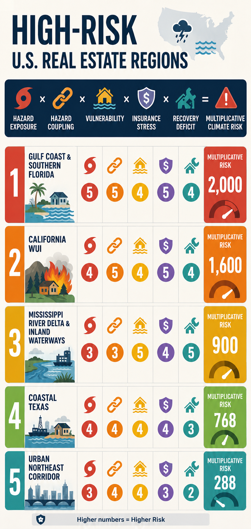
Hazard Exposure × Hazard Coupling × Vulnerability × Insurance Stress × Recovery Deficit = Multiplicative Climate Risk

Each component is scored from 1 to 5, where:

1 = Low Risk

2 = Moderate-Low Risk

3 = Moderate Risk

4 = High Risk

5 = Extreme Risk

The resulting score is not a probability of loss or a conventional actuarial measure. It is a comparative systems-risk index designed to identify locations where multiple weaknesses can reinforce one another.

This distinction is critical.

A region with a score of 5 in one category but relatively low scores elsewhere may be less systemically exposed than a region scoring 4 or 5 across nearly every category.

The multiplicative framework captures that interaction:

Physical Hazard ↑ + Coupling ↑ + Vulnerability ↑ + Insurance Stress ↑ + Recovery Capacity ↓ → Cascading Real-Estate Risk ↑↑

The following ranking represents a comparative assessment of major U.S. real-estate risk regions, incorporating physical hazards and the increasingly important financial and institutional dimensions of climate exposure.

1. Gulf Coast & Southern Florida

The Compound-Compounding Zone

Hazard Exposure — 5/5

The Gulf Coast and southern Florida face some of the country’s most concentrated combinations of acute and chronic climate hazards.

These include:

Major Hurricanes + Storm Surge + Extreme Rainfall + Sea-Level Rise + Coastal Flooding + Extreme Heat

The region’s vulnerability is not based on any single hazard. It is the convergence of multiple hazards affecting a densely developed coastal real-estate market.

Hazard Coupling — 5/5

The defining characteristic is the interaction among hazards.

A tropical cyclone can simultaneously produce:

Storm Surge + Extreme Rainfall + River Flooding + High Winds

Sea-level rise increases the baseline upon which storm surge occurs, while extreme rainfall can overwhelm drainage systems at the same time that elevated coastal water levels restrict drainage.

The resulting process is:

Hurricane → Storm Surge + Extreme Rainfall → Drainage Impairment → Compound Flooding → Widespread Property Exposure

This is precisely the type of coupled hazard that can produce disproportionate economic consequences.

Vulnerability — 4/5

The region contains enormous quantities of residential, condominium, commercial, and infrastructure assets exposed to coastal and flood hazards.

Building age and construction standards vary substantially. Newer construction and mitigation measures can reduce vulnerability, while older structures and properties with inadequate flood, wind, or drainage protection remain substantially more exposed.

The critical issue is therefore not simply the age of the housing stock, but the mismatch between:

Long-Lived Real Estate Assets → Rapidly Changing Climate Risk

Insurance Stress — 5/5

Insurance is one of the most consequential real-estate constraints in the region.

The combination of hurricanes, storm surge, flooding, wind damage, sea-level rise, and repeated catastrophe losses places substantial pressure on insurance availability and affordability.

The resulting feedback is:

Climate Risk ↑ → Expected Losses ↑ → Insurance Premiums ↑ → Deductibles and Coverage Restrictions ↑ → Insurance Availability ↓

For homeowners, insurance costs directly increase the cost of ownership.

For commercial real estate, rising insurance expenses can reduce net operating income and asset values by increasing operating costs. The effect is particularly significant for multifamily, hospitality, retail, and other income-producing properties.

The insurance problem therefore extends beyond individual policies.

It becomes a real-estate valuation problem:

Insurance Cost ↑ → Cost of Ownership ↑ → Buyer Demand ↓ → Property Values ↓

Recovery Deficit — 4/5

The region’s substantial public and private capital resources provide recovery capacity, but the scale of the infrastructure challenge is enormous.

Long-term pressures include:

Flood-Control Systems + Pump Stations + Drainage Networks + Seawalls + Roads + Bridges + Utilities + Wastewater Systems

The concern is not whether these systems can recover from one disaster.

The concern is whether:

Repeated Damage > Available Recovery and Adaptation Capacity

If the frequency of major events increases faster than infrastructure can be repaired, upgraded, or relocated, a recovery deficit can develop.

Multiplicative Risk

5 × 5 × 4 × 5 × 4 = 2,000

Total Risk Factor: 2,000

The Gulf Coast and southern Florida therefore represent the most pronounced example of compound climate-real-estate risk in the framework.

2. Central & Southern California Wildland-Urban Interface

The Fire–Flood–Insurance Cascade Zone

Hazard Exposure — 4/5

The Central and Southern California WUI faces a combination of:

Wildfire + Extreme Heat + Drought + Water Stress + Extreme Rainfall

The exposure is particularly consequential because enormous quantities of residential real estate have been constructed adjacent to or within wildfire-prone landscapes.

Hazard Coupling — 5/5

The defining feedback is:

Drought → Vegetation Stress → Wildfire → Vegetation Loss → Soil Destabilization → Extreme Rainfall → Mudslides and Debris Flows

This is a classic sequential compound-risk mechanism.

Wildfire does not simply produce immediate property losses.

It can alter the landscape in ways that increase the consequences of subsequent precipitation events.

The result is:

Wildfire → Landscape Transformation → Increased Post-Fire Flood/Mudslide Risk

This creates a risk cascade extending beyond the original fire.

Vulnerability — 4/5

Residential development in steep terrain, narrow canyons, and areas with constrained evacuation routes can create substantial exposure.

Vulnerability also depends on construction standards, defensible space, vegetation management, access routes, and the ability of communities to recover rapidly after catastrophic fires.

Insurance Stress — 5/5

California represents one of the clearest examples of insurance-market stress becoming a real-estate problem.

The combination of catastrophic wildfire exposure, rapidly changing risk conditions, and repeated losses creates pressure on insurers to increase premiums, restrict coverage, reduce exposure, or withdraw from high-risk markets.

When private insurance becomes unavailable or unaffordable, property owners may be forced into residual or state-backed insurance mechanisms.

The resulting feedback is:

Wildfire Risk ↑ → Insurance Losses ↑ → Premiums ↑ → Coverage Restrictions ↑ → Private Insurance Availability ↓ → Residual-Market Dependence ↑

This creates a second real-estate feedback:

Insurance Availability ↓ → Financing Constraints ↑ → Buyer Pool ↓ → Property Liquidity ↓ → Property Values ↓

The insurance problem can therefore become a leading indicator of broader real-estate repricing.

Recovery Deficit — 4/5

Large wildfire events can produce extensive reconstruction requirements simultaneously.

The recovery system must contend with:

Destroyed Housing + Infrastructure Damage + Debris Removal + Labor Requirements + Construction Demand + Supply Constraints

The resulting competition for labor and materials can extend rebuilding timelines and increase reconstruction costs.

The longer recovery takes, the greater the potential for:

Recovery Delay → Business Interruption → Household Displacement → Reduced Local Economic Activity → Reduced Community Resilience

Multiplicative Risk

4 × 5 × 4 × 5 × 4 = 1,600

Total Risk Factor: 1,600

The California WUI therefore represents a particularly important example of insurance availability becoming a leading indicator of real-estate climate risk.

3. Coastal Texas

The Industrial and Commercial Risk Hub

Hazard Exposure — 4/5

Coastal Texas faces:

Hurricanes + Storm Surge + Extreme Rainfall + Flash Flooding + Extreme Heat + Grid Stress

The region’s importance is amplified by its enormous concentration of industrial, commercial, petrochemical, port, logistics, and residential assets.

Hazard Coupling — 4/5

The physical hazards can interact through several pathways.

For example:

Extreme Heat → Electricity Demand ↑ → Grid Stress ↑ → Power Disruption → Cooling/Industrial/Commercial Disruption

At the same time:

Hurricane → Wind + Surge + Rainfall → Flooding + Power Loss → Business Interruption

And:

Flooding + Heat + Power Loss → Mold + Water Damage + Equipment Failure + Building-System Damage

This produces a multi-system cascade rather than a single flood loss.

Vulnerability — 4/5

Coastal Texas contains enormous concentrations of development and infrastructure in flood-prone and low-lying areas.

Impervious surfaces can increase runoff, while dense development can make drainage problems more consequential.

The concentration of industrial and commercial assets also creates correlated economic risk.

A single major event can affect multiple businesses, transportation systems, suppliers, utilities, and customers simultaneously.

Insurance Stress — 4/5

Insurance costs and coverage limitations are becoming an increasingly important component of real-estate risk.

Wind, hail, hurricane, flood, and business-interruption exposures can produce substantial premiums and deductibles.

As insurers reassess catastrophe exposure, property owners can increasingly absorb a greater portion of the risk through:

Higher Deductibles + Coverage Restrictions + Increased Premiums + Greater Self-Insurance

For commercial real estate, increasing insurance expenses directly affect:

Operating Expenses ↑ → NOI ↓ → Capitalization Value ↓

This provides a direct financial transmission mechanism between climate risk and commercial property valuation.

Recovery Deficit — 3/5

Coastal Texas possesses substantial private capital and strong economic capacity, which can accelerate reconstruction.

However, public infrastructure and regional systems can take much longer to repair.

The result is a two-speed recovery:

Private Capital → Rapid Property Recovery

while:

Public Infrastructure → Slower System Recovery

This creates a temporary resilience gap.

Multiplicative Risk

4 × 4 × 4 × 4 × 3 = 768

Total Risk Factor: 768

Coastal Texas represents an important example of how high-value commercial real estate can convert physical climate exposure into large-scale correlated financial losses.

4. Mississippi River Delta & Inland Waterways

The Structural-Aging and Recovery-Deficit Zone

Hazard Exposure — 3/5

The Mississippi Delta and associated inland waterways face:

River Flooding + Extreme Rainfall + Severe Convective Storms + Subsidence + Coastal Flooding

The region’s raw hazard exposure is lower than some Gulf Coast locations, but the interaction of hazards with infrastructure and socioeconomic vulnerability dramatically increases systemic risk.

Hazard Coupling — 3/5

One important pathway is:

Upstream Extreme Rainfall → River Discharge ↑ → Downstream Flooding → Prolonged Inundation → Structural and Infrastructure Damage

In coastal portions of the Delta, this can interact with:

River Flooding + Storm Surge + Sea-Level Rise → Compound Inland/Coastal Flooding

The duration of inundation can be as important as peak water depth because prolonged water exposure can increase mold, structural deterioration, electrical damage, and infrastructure failure.

Vulnerability — 5/5

This region’s primary vulnerability is structural.

Risk is amplified by:

Aging Infrastructure + Levee Dependence + Aging Buildings + Economic Constraints + Limited Local Fiscal Capacity

The critical issue is not simply whether flood-control infrastructure exists.

It is whether that infrastructure can be maintained, upgraded, and replaced at the rate required under changing climate conditions.

Insurance Stress — 4/5

Flood insurance is an essential component of property financing in designated high-risk areas where federal requirements apply.

However, the availability and affordability of private flood coverage can vary substantially by location and risk profile.

Where private coverage is limited, property owners can become increasingly dependent on federal flood insurance and other residual mechanisms.

This creates another form of concentration risk:

Private Insurance Capacity ↓ → Public Backstop Dependence ↑

The problem becomes more acute when repeated losses increase premiums, deductibles, or coverage restrictions faster than property values and household incomes can absorb them.

Recovery Deficit — 5/5

This is the region’s defining weakness.

A major flood can produce:

Property Damage → Income Loss → Reduced Local Tax Revenue → Infrastructure Damage → Limited Local Recovery Capacity

Federal disaster assistance can be essential, but administrative processes, funding requirements, and reconstruction complexity can extend recovery timelines.

The resulting feedback can become:

Low Local Fiscal Capacity → Slow Recovery → Persistent Damage → Lower Property Values → Lower Tax Base → Even Lower Recovery Capacity

Multiplicative Risk

3 × 3 × 5 × 4 × 5 = 900

Total Risk Factor: 900

This produces an important result:

The Mississippi Delta scores lower than Coastal Texas in raw hazard exposure but higher in total multiplicative risk.

That is precisely why a multiplicative framework is useful.

A moderate physical hazard can produce extreme systemic risk when combined with high vulnerability and a severe recovery deficit.

5. Urban Northeast Corridor

The Legacy-Infrastructure and Urban-Flooding Zone

Hazard Exposure — 3/5

The urban Northeast faces:

Nor’easters + Extreme Rainfall + Tidal Flooding + Sea-Level Rise + Urban Flash Flooding

The region does not necessarily experience the most extreme individual climate hazards in the country.

Its risk derives from density, infrastructure age, and enormous concentrations of economic value.

Hazard Coupling — 4/5

A central pathway is:

Sea-Level Rise → Higher Coastal Baseline → Reduced Stormwater Drainage Capacity → Heavy Rainfall → Urban Flooding

The resulting flooding can affect:

Basements + Subways + Tunnels + Electrical Systems + Transportation Networks + Commercial Districts

This creates a particularly important urban cascade:

Extreme Rainfall → Stormwater Overload → Transit Disruption → Workforce Disruption → Business Interruption → Economic Loss

Vulnerability — 4/5

The region contains extraordinary quantities of legacy infrastructure and older real estate.

Many structures were designed under climate conditions substantially different from those now emerging.

Below-grade spaces can be especially vulnerable:

Basement Housing + Electrical Rooms + Subway Infrastructure + Underground Transportation

This makes the region highly sensitive to intense precipitation even when properties are not located directly adjacent to rivers or coastlines.

Insurance Stress — 3/5

Insurance remains more available than in the most stressed coastal and wildfire markets, but the trajectory remains important.

Increasing flood claims, basement losses, storm damage, and infrastructure disruption can gradually increase premiums and deductibles.

The principal concern is therefore not an immediate insurance-market collapse but gradual repricing of urban climate exposure.

The feedback is:

Urban Flood Risk ↑ → Claims ↑ → Insurance Costs ↑ → Cost of Ownership ↑ → Property-Value Pressure ↑

Recovery Deficit — 2/5

The Northeast possesses comparatively strong municipal tax bases, financial resources, infrastructure institutions, and access to federal resources.

This provides substantial recovery capacity.

However, the scale and age of infrastructure create long-term adaptation challenges.

The region’s primary weakness is therefore not immediate recovery capacity but the enormous cost of modernizing legacy systems before they become repeatedly overwhelmed.

Multiplicative Risk

3 × 4 × 4 × 3 × 2 = 288

Total Risk Factor: 288

The Urban Northeast demonstrates that high population density and high property values do not automatically produce the highest multiplicative risk.

Strong fiscal and institutional recovery capacity can substantially reduce systemic risk.

Real-Estate Climate Risk Comparison Matrix

The following matrix applies the five-factor multiplicative framework:

Region	Hazard Exposure	Hazard Coupling	Vulnerability	Insurance Stress	Recovery Deficit	Multiplicative Risk
1. Gulf Coast & Southern Florida	5	5	4	5	4	2,000
2. California WUI	4	5	4	5	4	1,600
3. Mississippi River Delta & Inland Waterways	3	3	5	4	5	900
4. Coastal Texas	4	4	4	4	3	768
5. Urban Northeast Corridor	3	4	4	3	2	288

Why the Ranking Matters

The ranking demonstrates why climate-driven real-estate risk cannot be measured solely by the severity of weather.

The Mississippi Delta provides the clearest example.

Its 3/5 hazard-exposure score is lower than Coastal Texas’s 4/5, yet its overall multiplicative score is higher:

Mississippi Delta → 900

Coastal Texas → 768

The difference arises from the interaction of:

High Vulnerability + High Insurance Stress + Severe Recovery Deficit

This is the essence of cascading risk.

A region does not need to have the most extreme weather to have the greatest systemic vulnerability.

It needs to have the most dangerous combination of interacting weaknesses.

The Central Insurance Feedback

Across the five regions, insurance functions as one of the primary transmission mechanisms connecting physical climate risk to real-estate values.

The feedback can be represented as:

Climate Risk ↑ → Expected Losses ↑ → Insurance Claims ↑ → Premiums ↑ → Deductibles ↑ → Coverage Restrictions ↑ → Insurance Availability ↓ → Cost of Ownership ↑ → Property Demand ↓ → Property Values ↓

Once property values begin declining, another feedback can emerge:

Property Values ↓ → Mortgage Collateral ↓ → Lending Risk ↑ → Financing Constraints ↑ → Buyer Pool ↓ → Property Liquidity ↓ → Property Values ↓

Insurance therefore does not merely compensate property owners after losses.

It can influence whether a property can be:

Owned → Financed → Sold → Developed → Maintained → Insured

This makes insurance availability and affordability a critical component of real-estate climate risk.

The Major Coupled Feedback Loops

1. Insurance–Property Value Feedback

Climate Risk ↑ → Insurance Losses ↑ → Premiums ↑ / Availability ↓ → Cost of Ownership ↑ → Buyer Demand ↓ → Property Values ↓

2. Property Value–Tax Base Feedback

Property Values ↓ → Tax Base ↓ → Municipal Revenue ↓ → Infrastructure Investment ↓ → Resilience ↓ → Flood Risk ↑ → Property Values ↓

3. Recovery-Deficit Feedback

Disaster Frequency ↑ → Recovery Window ↓ → Unresolved Damage ↑ → Vulnerability ↑ → Next-Event Losses ↑ → Recovery Window ↓

4. Insurance–Mortgage Feedback

Physical Risk ↑ → Insurance Stress ↑ → Coverage Constraints ↑ → Mortgage Risk ↑ → Lending Constraints ↑ → Buyer Pool ↓ → Property Values ↓

5. Commercial Real-Estate Feedback

For income-producing properties:

Climate Risk ↑ → Insurance + Maintenance + Adaptation Costs ↑ → Operating Expenses ↑ → NOI ↓ → Property Value ↓

This relationship is particularly important for multifamily, hospitality, retail, industrial, and other income-producing properties.

The Cascading Real-Estate Framework

The five regional examples reveal several recurring stages in the emerging climate-real-estate cascade:

Physical Hazard

Warming → Sea-Level Rise + Heavier Rainfall + Stronger/Slower Storms + Extreme Heat + Drought

Hazard Coupling

Multiple Hazards → Compound Events → Greater Physical Exposure

Property Damage

Compound Hazard → Structural Damage + Infrastructure Damage + Business Interruption

Insurance Stress

Losses ↑ → Premiums ↑ + Deductibles ↑ + Coverage Restrictions ↑ + Availability ↓

Property Repricing

Insurance Cost ↑ → Cost of Ownership ↑ → Buyer Demand ↓ → Property Values ↓

Financial Amplification

Property Values ↓ → Mortgage Risk ↑ + Investment ↓ + Liquidity ↓

Municipal Amplification

Property Values ↓ → Tax Base ↓ → Infrastructure Investment ↓

Resilience Erosion

Infrastructure Investment ↓ + Recovery Capacity ↓ → Vulnerability ↑

Cascading Risk

Vulnerability ↑ → Future Losses ↑ → Insurance Stress ↑ → Property Values ↓

The resulting closed-loop system is:

Climate Hazard → Physical Loss → Insurance Stress → Property-Value Decline → Investment Decline → Tax-Base Erosion → Infrastructure Deterioration → Recovery Deficit → Greater Vulnerability → Greater Future Loss

The Central Finding

The Multiplicative Climate Risk framework produces a fundamentally different understanding of climate-exposed real estate.

The highest-risk region is not necessarily the region with:

The Most Hurricanes

The Most Wildfires

The Most Rainfall

The Highest Sea-Level Rise

Instead, it is the region where multiple risk factors interact:

Hazard Exposure × Hazard Coupling × Vulnerability × Insurance Stress × Recovery Deficit

The resulting system can become self-reinforcing:

Climate Hazard → Insurance Stress → Property-Value Decline → Investment Decline → Tax-Base Erosion → Infrastructure Resilience Decline → Recovery Deficit → Greater Vulnerability → Greater Future Loss

This is the central transition from climate hazard to cascading real-estate risk.

The most consequential property-market question is therefore no longer simply:

Will this property flood, burn, or be damaged by extreme weather?

It is:

Can this property remain insurable, financeable, valuable, maintainable, and economically viable as climate hazards become more frequent and increasingly coupled?

That question shifts climate-risk analysis from the physical event itself to the long-term resilience of the economic system surrounding the property.

And that is where the greatest risks may emerge.

The weather creates the shock.
Coupled hazards amplify the shock.
Insurance translates the shock into financial cost.
Real estate capitalizes the cost into property values.
Weak recovery capacity allows the damage to accumulate.
And cascading feedbacks can turn a climate hazard into a real-estate crisis.

Wildfire Catastrophe Bonds Surge as Insurers Transfer Record Climate Risk to Capital Markets

Posted on 2026/08/052026/08/06 by admin

by Sidd Mukherjee and Daniel Brouse

A New Era of Climate Risk Finance

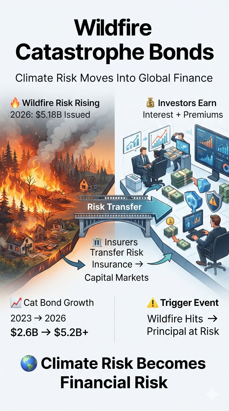
Wildfire-exposed catastrophe bond issuance has surged to $5.183 billion year-to-date in 2026, rapidly approaching the full-year record of $5.55 billion set in 2025. Driven by escalating wildfire losses, expanding climate risks, and increasingly sophisticated risk models, insurers are turning to global capital markets to transfer unprecedented levels of wildfire exposure.

Catastrophe bonds—often called cat bonds—allow insurers and governments to shift extreme disaster risks away from traditional insurance markets and onto investors. Investors receive attractive returns if a defined catastrophe does not occur, but may lose some or all of their principal if a triggering event causes significant losses.

The rapid growth of wildfire-linked cat bonds reflects a fundamental shift: wildfire is no longer viewed as a regional insurance problem but as a major global financial risk.

Wildfire Cat Bond Issuance Reaches Historic Levels

According to data compiled by Artemis, wildfire-related risk capital has experienced dramatic multi-year growth:

2023: $2.57 billion issued
2024: $2.84 billion issued
2025: Record $5.55 billion issued
2026 (year-to-date): $5.183 billion issued

The acceleration reflects rising insured wildfire losses, increasing pressure on traditional insurers, and investor demand for alternative assets that are not closely correlated with stocks and bonds.

Wildfire Risk Becomes a Major Alternative Asset Class

From Niche Exposure to Global Investment Market

Wildfire risk is rapidly evolving from a specialized insurance concern into a standalone catastrophe-risk asset class. Investors are increasingly attracted to catastrophe bonds because disaster events generally have little relationship to traditional financial markets.

Unlike stocks, bonds, or commodities, catastrophe bonds are driven primarily by physical climate events rather than economic cycles.

Advanced Climate Risk Modeling

Improved modeling capabilities have increased investor confidence. Companies such as Verisk and Moody’s have developed increasingly sophisticated catastrophe models that incorporate updated climate data, changing fire behavior, and evolving exposure patterns.

These models help investors evaluate wildfire probability, potential losses, and appropriate risk premiums.

Human Mitigation Changes the Risk Equation

Wildfire risk differs from many natural hazards because human actions can influence outcomes. Measures such as vegetation management, defensible space creation, utility improvements, and community fire planning can alter expected losses and affect catastrophe bond risk assessments.

Key Sponsors and Expanding Markets

California FAIR Plan Returns to the Cat Bond Market

California’s insurer of last resort, the California FAIR Plan, returned to the catastrophe bond market through the Golden Bear Re Ltd. Series 2026-2 transaction, successfully raising its target to $400 million.

The move highlights the growing difficulty of relying solely on traditional insurance markets in regions facing persistent wildfire threats.

Mercury General Targets Fire Risk Transfer

Mercury General Corporation sponsored the Luca Re Ltd. Series 2026-1 catastrophe bond transaction, targeting $150 million in fire-related reinsurance protection.

European Insurers Explore Wildfire Risk Transfer

Although wildfire catastrophe bond issuance remains heavily concentrated in California, increasingly severe wildfire seasons are pushing European insurers to explore capital-market solutions and alternative risk-transfer structures.

How Catastrophe Bonds Work

A catastrophe bond transfers disaster risk from an insurer to investors.

The insurer pays investors a premium for assuming the risk. Investors receive regular interest payments, but their principal is placed at risk if a predefined catastrophe occurs.

How Investors Make Money

1. Regular Interest Payments

Investors receive monthly or quarterly coupon payments that compensate them for accepting catastrophe exposure.

2. Risk Premium Spread

Sponsors pay an elevated interest spread because investors are taking on the possibility of losing principal.

3. Collateral Yield

The invested principal is typically held in a secure collateral account that generates additional low-risk interest income.

4. Total Return

The investor’s return combines the catastrophe bond premium spread and collateral investment yield.

How Investors Can Lose Their Principal

Binary Catastrophe Risk

If a wildfire reaches the bond’s predetermined trigger conditions, investors may lose part or all of their principal.

Immediate Capital Transfer

When triggered, the lost principal is transferred to the insurance sponsor to help cover wildfire claims.

No Insurance Company Default Required

Unlike traditional corporate bonds, investors do not lose money because an insurer fails financially. The catastrophe itself triggers the loss.

Full Return Without Trigger

If no qualifying wildfire occurs during the bond term—typically three to five years—the investor receives the full principal back at maturity.

How Wildfire Cat Bond Triggers Work

Indemnity Triggers

Payments are based on the sponsor’s actual insured losses from a wildfire event.

Example: An insurer suffers billions of dollars in wildfire claims, triggering payment from the catastrophe bond.

Parametric Triggers

Payments are based on measurable physical conditions rather than financial losses.

Examples:

Acres burned
Fire intensity
Geographic location
Wind conditions
Temperature thresholds

Industry Loss Triggers

Payments are based on total insurance industry losses from a catastrophe, calculated by independent organizations such as catastrophe loss index providers.

Climate Risk Moves Into Global Finance

The rapid expansion of wildfire catastrophe bonds signals a major transformation in how society manages climate risk. As extreme wildfire seasons become more frequent and expensive, insurers are increasingly relying on financial markets to absorb losses that traditional insurance systems can no longer easily contain.

Wildfire risk is becoming not only an environmental challenge but also a major test of global financial resilience.

The Major Perils Behind the Global Catastrophe Bond Market

Tropical cyclones and earthquakes remain the two foundational pillars of the global catastrophe bond market, traditionally accounting for a large share of the roughly $65.6 billion in outstanding risk capital. Wildfire, however, has rapidly expanded into a significant standalone risk category as insurers confront escalating losses and growing climate exposure.

The catastrophe bond market now spans a broad spectrum of natural, human-caused, and emerging systemic risks.

Core Property Perils

Tropical Cyclones — Hurricanes and Typhoons
Tropical cyclones are among the largest sources of catastrophe bond risk. Coverage is concentrated in U.S. hurricanes, particularly along Florida, the Gulf Coast, and the Eastern Seaboard, as well as Japanese typhoons and Australian cyclones.

Earthquakes
Earthquake risk represents one of the longest-established and most consistently modeled catastrophe bond perils. Major exposure centers include California, the Pacific Northwest, Japan, and New Zealand, where severe seismic events can generate enormous insured losses.

Severe Convective Storms
This increasingly important category covers highly localized but frequent atmospheric hazards, including tornadoes, severe hail, and straight-line winds such as derechos. Repeated losses from these events have become a significant source of claims for U.S. property insurers.

Wildfires
Wildfire has rapidly evolved from a relatively specialized exposure into a major standalone catastrophe bond peril. California remains the dominant market, but growing wildfire losses are driving interest in risk-transfer solutions across other regions.

Winter Storms and Floods
Catastrophe bonds can also protect insurers against extreme winter weather, including freezing events, heavy snowfall, ice damage, and infrastructure failures, as well as coastal and inland flooding.

Emerging and Specialized Perils

Cyber Risk
Cyber catastrophe bonds are an emerging non-natural peril designed to protect insurers against systemic cyber events. Potential triggers include widespread cloud-service disruptions, ransomware attacks, or failures of critical digital infrastructure.

Life, Health, and Mortality Risk
Life and health catastrophe securities can transfer the risk of sudden, extreme increases in mortality or health-related losses. Pandemic-scale events represent one potential source of catastrophic exposure.

Operational and Terrorism Risk
Specialized catastrophe structures have also been used to transfer extreme human-caused risks, including terrorism and major operational disruptions affecting businesses, infrastructure, or public institutions.

Multi-Peril vs. Standalone Catastrophe Bonds

Catastrophe bonds do not always cover a single peril. Many transactions combine several risks into a multi-peril structure, allowing insurers to diversify their exposure and potentially provide investors with a broader risk profile.

For example, a single transaction may combine U.S. named storms, earthquakes, severe convective storms, and wildfire under one bond.

This structure is important because catastrophe bonds can function much like a portfolio of climate and disaster risks: investors are exposed to multiple potential events, while insurers gain protection against losses that could otherwise overwhelm traditional reinsurance capacity.

A Market Expanding Beyond Traditional Disasters

The evolution of the catastrophe bond market reflects a broader transformation in global risk. What began primarily as a mechanism for transferring hurricane and earthquake risk has expanded into a sophisticated financial system capable of pricing and transferring exposure to wildfires, severe storms, floods, cyberattacks, pandemics, and other low-probability, high-impact events.

As climate change increases the frequency, severity, geographic reach, or financial consequences of certain extreme events, catastrophe bonds are becoming an increasingly important bridge between physical risk, insurance markets, and global investment capital.

Climate Change Impacts and You: The Rising Cost of a Changing Climate

Posted on 2026/08/042026/08/04 by admin

by Daniel Brouse

Introduction

Climate change is no longer simply a future environmental threat. It is increasingly affecting American households through higher costs, declining air quality, extreme heat, infrastructure disruptions, property damage, and changing patterns of disease.

Although catastrophic floods, hurricanes, wildfires, and other disasters dominate the headlines, the most widespread climate impact may be less dramatic: the steady financial pressure climate change places on everyday household budgets. Food prices, insurance premiums, utility bills, and the costs of maintaining homes and communities are all increasingly influenced by a changing climate.

The impacts are not distributed equally. Some are nearly universal, while others are concentrated in particular regions or communities. The ranking below therefore considers two factors: how widely households are exposed and how severely the impact can disrupt everyday life.

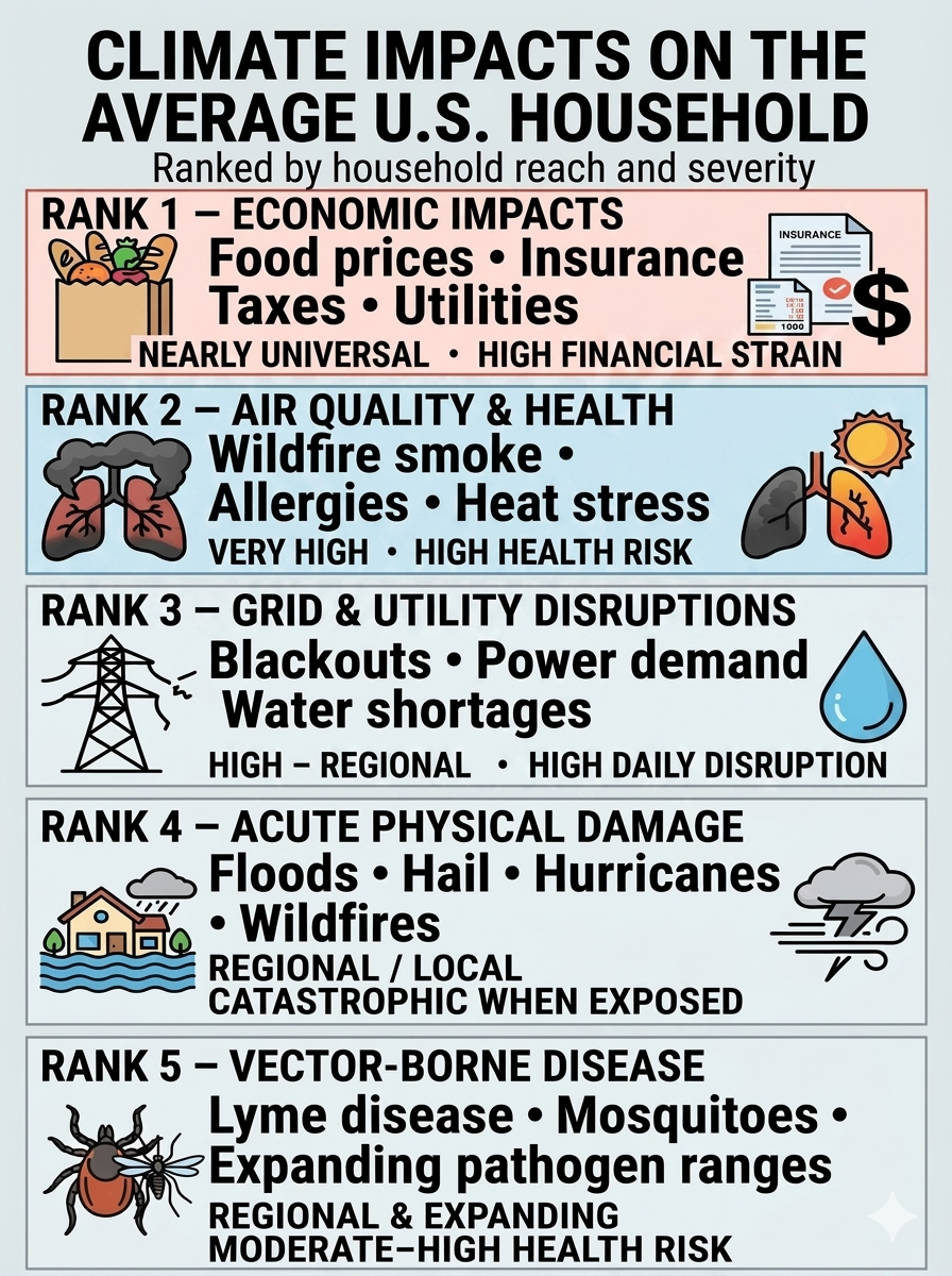
Ranking of Climate Impacts on the Average U.S. Household

Rank	Impact Category	Primary Household Threats	Ubiquity	Severity
1	Economic Impacts	Food inflation, insurance premiums, taxes, utility costs	Nearly universal	High financial strain
2	Air Quality & Chronic Health	Wildfire smoke, longer allergy seasons, heat stress	Very high	High health risk
3	Grid & Utility Disruptions	Blackouts, heat-related demand, water shortages	High, but regional	High daily disruption
4	Acute Physical Damage	Floods, hail, hurricanes, wildfires	Regional/local	Catastrophic when exposed
5	Vector-Borne Diseases	Lyme disease, mosquitoes, expanding pathogen ranges	Regional and expanding	Moderate to high health risk

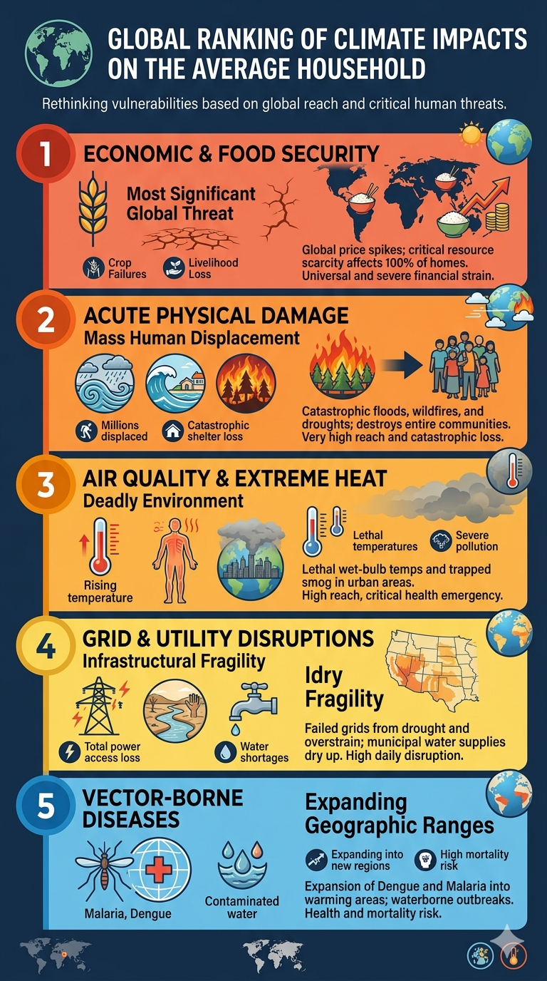
Global Ranking of Climate Impacts on the Average Household

The ranking below shifts the order of impacts based on global reach and the immediate threat to human life and livelihoods across developing and developed nations alike.

Rank	Impact Category	Primary Global Household Threats	Ubiquity	Severity
1	Economic & Food Security	Global food price spikes, crop failures, loss of agricultural livelihoods	Universal (100% of homes)	Extreme financial/survival strain
2	Acute Physical Damage	Catastrophic monsoon flooding, sea-level rise, mega-wildfires, historic droughts	Very High (Millions displaced)	Catastrophic loss of shelter
3	Air Quality & Extreme Heat	Lethal wet-bulb temperatures, severe dust/smoke pollution, urban heat islands	High (Equatorial & Urban zones)	Critical health emergency
4	Grid & Utility Disruptions	Total lack of power access, severe municipal water shortages, drying river basins	High (Varies by infrastructure)	High daily survival disruption
5	Vector-Borne Diseases	Malaria, Dengue fever expansion, waterborne cholera outbreaks	Expanding (Sub-tropical regions)	High health and mortality risk

1. Economic Impacts: The Most Universal Climate Burden

Economic impacts rank first because households do not have to live in a flood zone, wildfire corridor, or hurricane-prone region to pay the economic costs of climate change. Climate-related costs increasingly reach Americans through food prices, insurance premiums, utility bills, taxes, public fees, and the rising cost of maintaining homes and infrastructure.

Climate change can therefore function as a cost multiplier, increasing expenses both directly and indirectly.

Climate-Driven Food Inflation

Drought, extreme heat, excessive rainfall, and other weather disruptions can reduce agricultural yields and interfere with food production and supply chains. Because food markets are interconnected, production losses in one region can influence prices far beyond the location of the original climate event.

The effects can reach everyday staples and commodities such as coffee, wheat, corn, beef, fruits, and vegetables.

The result is a climate-related cost that can reach virtually every household through the grocery bill—even when the household is hundreds or thousands of miles from the drought, flood, or heatwave affecting agricultural production.

The Insurance Crisis

Insurance is one of the clearest mechanisms through which climate risk is transferred directly to households.

As floods, hurricanes, wildfires, severe storms, and other disasters generate increasingly costly losses, insurers may respond by raising premiums, increasing deductibles, restricting coverage, or withdrawing from particularly high-risk markets.

For homeowners, climate risk can therefore produce a double financial burden:

higher insurance costs + higher uninsured exposure.

In some locations, the problem extends beyond affordability. Homeowners may find that certain types of coverage are difficult or impossible to obtain through conventional private insurance markets.

Rising Utility Costs

Hotter summers increase demand for air conditioning. As temperatures remain elevated for longer periods, households may need to run cooling systems more frequently and for longer durations.

That increases electricity consumption while simultaneously placing additional stress on the power grid.

Climate change can therefore affect household budgets through both higher energy consumption and the cost of maintaining a more resilient electrical system.

Water systems can face similar pressures. Drought, declining water supplies, flooding, and changing precipitation patterns may require communities to invest in new reservoirs, treatment capacity, pipelines, drainage systems, and other infrastructure.

Those investments ultimately have to be paid for.

Taxes, Assessments, and Public Costs

One of the least visible climate costs is the portion that reaches households through government budgets rather than private markets.

When climate-related disasters become more costly, governments must spend more on emergency response, disaster recovery, infrastructure repair, flood protection, stormwater management, wildfire preparedness, water systems, coastal protection, and long-term climate adaptation.

Those expenses can eventually reach households through:

Property taxes used to finance infrastructure repairs and resilience projects.
Special assessments and municipal fees for stormwater, drainage, flood control, and other local projects.
Higher utility rates needed to upgrade vulnerable water and electrical systems.
State and federal taxes that help finance disaster recovery, emergency response, agricultural assistance, infrastructure rebuilding, and resilience programs.
Public insurance and disaster programs when private insurance markets cannot absorb the full cost of catastrophic losses.

This creates an important economic chain:

Climate hazard → physical damage → insurance losses → government response → infrastructure spending → taxes, fees, and utility costs.

The household may never experience the original flood, wildfire, hurricane, or drought, yet it can still participate in paying the bill.

Rising Property and Maintenance Costs

Climate stress can also increase the cost of owning and maintaining a home.

More intense rainfall can require improved drainage. Stronger storms can increase demand for roofing and exterior repairs. Heat can accelerate deterioration of infrastructure and building materials. Flooding and wildfire risk can require additional mitigation measures.

At the same time, widespread disasters can create temporary shortages of construction materials, contractors, equipment, and skilled labor, increasing repair costs.

The Hidden Climate Cost

Taken together, these effects mean that climate change does not have to destroy your home to affect your household finances.

A household can experience climate-related costs through:

Higher grocery prices
Higher insurance premiums
Higher electricity and water bills
Higher taxes and public fees
Higher repair and maintenance costs

Together, these expenses create a growing household climate burden—even when a family never experiences a major climate disaster firsthand.

The important point is that climate change is not simply a collection of isolated disasters. It is increasingly an economic force that propagates through markets, insurance systems, government budgets, and household expenses.

For the average American household, this may ultimately be the most widespread way climate change is experienced: not as one catastrophic event, but as a persistent accumulation of additional costs.

2. Air Quality & Chronic Health: A Widespread Physical Exposure

Climate change also affects the quality of the air people breathe.

Wildfire Smoke

Wildfire smoke can travel hundreds or even thousands of miles, carrying fine particulate matter such as PM₂.₅ into communities far from the original fire.

These particles can penetrate deep into the respiratory system and aggravate existing respiratory and cardiovascular problems. As wildfire activity and smoke exposure increase in some regions, air-quality impacts are no longer limited to communities immediately adjacent to fires.

Longer Allergy Seasons

Warmer temperatures can alter plant growing seasons and extend periods of pollen production.

For people with asthma or seasonal allergies, longer or more intense pollen seasons can mean more days of symptoms, greater medication use, and reduced quality of life.

Heat Stress

Rising baseline temperatures also increase the frequency and duration of dangerous heat.

Homes without adequate cooling, outdoor workplaces, and communities with limited access to cooling resources can be particularly vulnerable. Extreme heat is not merely uncomfortable—it can place substantial physiological stress on the human body.

3. Grid & Utility Disruptions: Climate Stress on Essential Infrastructure

Modern households depend on electricity, water, transportation, telecommunications, and other infrastructure every day.

Climate extremes can place additional stress on these systems.

Power Grid Failures

Extreme heat can push electricity demand toward peak levels as households and businesses increase air-conditioning use.

At the same time, extreme weather can damage transmission lines, substations, transformers, and other infrastructure.

The consequences can range from higher electricity costs to localized outages and, under severe conditions, prolonged disruptions to essential services.

Water Scarcity

Drought can reduce reservoir levels, groundwater availability, and other sources of municipal water.

Communities may respond with conservation requirements, watering restrictions, infrastructure investments, or higher water costs.

Water stress can therefore become both an environmental problem and a household financial problem.

4. Acute Physical Damage: Catastrophic Where It Strikes

Floods, hurricanes, wildfires, severe thunderstorms, hail, and high winds can cause enormous damage to homes, vehicles, businesses, and infrastructure.

This category ranks fourth not because the damage is minor, but because exposure is geographically concentrated.

A household directly hit by a major disaster can experience losses vastly greater than those associated with ordinary climate-related inflation.

Floods and Flash Floods

Intense rainfall can overwhelm drainage systems and produce rapid flooding in locations that may not have traditionally been considered high-risk.

Coastal communities also face storm surge and rising sea levels that can increase the consequences of major storms.

Severe Hail and Wind

Severe convective storms can produce damaging hail and straight-line or tornadic winds.

Roofing, siding, windows, vehicles, and other property can be damaged within minutes, creating repair costs that are often compounded by rising construction and insurance expenses.

Wildfires

Wildfires can destroy homes and communities directly while also creating secondary effects through smoke, evacuation, infrastructure disruption, and insurance losses.

5. Vector-Borne Diseases: A Smaller but Expanding Risk

Climate change can also alter the geographic range and seasonal activity of disease-carrying organisms.

Tick-Borne Illnesses

Changes in temperature and seasonal conditions can affect the distribution and activity of ticks and their hosts.

In some regions, this may increase opportunities for exposure to Lyme disease and other tick-borne illnesses.

Mosquito-Borne Diseases

Changing temperature and precipitation patterns can also influence mosquito populations and the geographic conditions suitable for certain mosquito-borne diseases.

The importance of this category varies considerably by region, but changing environmental conditions can alter the boundaries of disease risk over time.

Other Pathogens

Environmental changes can also affect exposure to less common infectious diseases, including tularemia (rabbit fever), which can be transmitted through several pathways involving ticks, biting flies, infected animals, or contaminated environments.

The Basics: How Climate Change Reaches Your Household

Climate change may seem like a global-scale phenomenon, but its consequences increasingly arrive through very ordinary parts of daily life.

Your Wallet: A Rising Cost of Living

Climate change can function like a hidden cost multiplier, increasing expenses directly and indirectly.

Higher grocery bills: Weather extremes can disrupt agricultural production and food supply chains.
Higher insurance premiums: Increasing disaster losses can raise premiums, deductibles, and coverage costs.
Higher utility bills: Hotter temperatures increase cooling demand and electricity consumption.
Higher repair costs: Disasters can increase demand for construction materials, contractors, and replacement vehicles.
Higher infrastructure costs and taxes: Communities may need to spend more on flood protection, stormwater systems, water supplies, roads, and electrical infrastructure.

The result is that climate change does not need to destroy your house to affect your household finances.

Your Health: New Physical Strains

A warmer climate can change the environmental conditions in which people live.

Extended Allergy Seasons

Longer growing seasons and changing pollen patterns can increase exposure for people with seasonal allergies and asthma.

Heat Stress

More frequent and intense heat events increase risks of heat exhaustion, heatstroke, dehydration, and other heat-related illnesses.

Air Pollution

Wildfire smoke and other climate-related air-quality problems can expose people to unhealthy concentrations of fine particulate matter.

Vector-Borne Disease

Changing environmental conditions can alter the geographic and seasonal ranges of ticks, mosquitoes, and other disease vectors.

Your Environment: Infrastructure and Safety

Climate change also affects the physical systems surrounding your home.

Property Damage

Flooding, severe storms, wildfires, hail, and high winds can damage homes, vehicles, and personal property.

Travel Disruptions

Flooded roads, damaged bridges, severe storms, wildfire smoke, and extreme heat can disrupt transportation and cause delays.

Power and Water Reliability

Extreme heat, drought, storms, and other hazards can put additional pressure on electricity and water systems.

These disruptions can affect people even when their own property escapes direct physical damage.

What You Can Do

Climate change is a global problem, but households can take practical steps to reduce both personal vulnerability and unnecessary expense.

Audit Home Energy

Improve insulation, use efficient lighting and appliances, and manage heating and cooling more efficiently.

Prepare for Emergencies

Maintain a basic emergency kit, understand local flood and wildfire risks, and have a plan for prolonged power outages.

Protect Your Property

Keep gutters and drainage systems clear, maintain trees and vegetation around structures, and understand your property’s exposure to flooding, wind, wildfire, and other hazards.

Reduce Waste

Reducing food waste, conserving water, and using energy efficiently can lower household costs while reducing resource demand.

Know Your Insurance

Review deductibles, exclusions, flood coverage, and other policies before disaster strikes. Standard homeowners insurance does not necessarily cover every major climate-related hazard.

The Bottom Line

Climate change is often discussed in terms of distant environmental consequences, but for American households, the most immediate effects are increasingly personal and financial.

You may encounter climate change as:

a higher grocery bill,
a larger insurance premium,
a higher electric bill,
a smoky summer afternoon,
a longer allergy season,
a power outage,
a flooded road,
a damaged roof,
or a greater risk of heat stress.

The most dramatic climate disasters will continue to make the headlines. But the deeper transformation may be quieter: climate change is becoming embedded in the ordinary economics and infrastructure of everyday life.

The question is no longer simply what will climate change do to the planet?

It is increasingly:

What will climate change cost you?

Climate Change and the Global Insurance Crisis: Rising Losses, Retreating Insurers, and the Growing Protection Gap

Posted on 2026/08/032026/08/03 by admin

by Daniel Brouse

Climate change is fundamentally destabilizing insurance markets by driving increasingly severe financial losses, pushing premiums sharply higher, and causing insurers to reduce or withdraw coverage in some high-risk regions. As extreme weather events become more frequent and, in many cases, more intense, traditional underwriting models are being challenged by rapidly changing risk. The result is a growing transfer of financial risk from private insurers to consumers, businesses, lenders, and governments.

The Protection Gap Crisis

One of the clearest signs of growing insurance instability is the widening protection gap—the difference between total economic losses from disasters and the portion covered by insurance.

In many climate-vulnerable regions, the majority of disaster losses remain uninsured. The gap can be particularly severe in developing economies, where insurance penetration is low and households, businesses, and governments may lack the financial resources to recover from catastrophic events.

This creates a dangerous feedback loop:

More extreme losses → higher insurance costs → reduced coverage → greater uninsured losses → greater financial vulnerability

The protection gap is therefore not simply an insurance problem. It is increasingly a problem of household financial security, economic resilience, infrastructure recovery, and public finance.

Corporate Pullbacks From High-Risk Regions

Insurers are increasingly reassessing their exposure to regions where climate-related risks are becoming more difficult to price and manage.

In some high-risk markets, major insurers have stopped writing certain types of new business, declined to renew policies, restricted coverage, increased deductibles, or imposed substantially higher premiums. These trends have been especially visible in wildfire-prone areas of California and hurricane- and flood-exposed coastal regions.

When private carriers retreat, governments and state-sponsored insurance programs often become insurers of last resort. This can concentrate risk in public or quasi-public systems while leaving taxpayers increasingly exposed to catastrophic losses.

Systemic Financial Risks

Mortgage Market Threats

Property insurance is closely connected to the housing and banking systems because mortgage lenders generally require borrowers to maintain adequate insurance on the underlying property.

As premiums rise and coverage becomes more difficult to obtain, homeowners can face rapidly increasing housing costs even when their mortgage payment remains unchanged. In the most exposed markets, some properties may become effectively uninsurable or prohibitively expensive to insure.

This creates a potential chain reaction:

Climate risk → higher insurance costs → declining property affordability → falling property values → mortgage stress → increased financial-system risk

The burden can fall disproportionately on lower-income homeowners, who have less capacity to absorb sudden increases in insurance and other climate-related costs.

Macroeconomic Volatility

Rising insurance premiums can also contribute to broader economic volatility. Insurance is an input into housing, transportation, agriculture, construction, business operations, and investment.

When insurers raise premiums to reflect increased catastrophe risk, those costs can eventually be passed through to consumers in the form of higher rents, housing costs, food prices, transportation costs, and prices for other goods and services.

In particularly vulnerable areas, insurance costs can also influence where people are willing and able to live. If housing becomes prohibitively expensive to insure—or insurance becomes unavailable altogether—households and businesses may begin relocating toward less exposed regions.

Climate change can therefore contribute to climate-driven migration within countries and across regions, even before an area becomes physically uninhabitable.

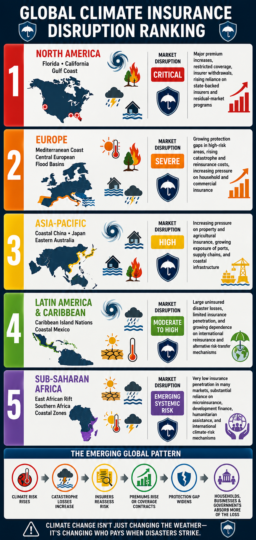
Global Climate Insurance Disruption Ranking

The global property and casualty (P&C) insurance market is experiencing very different levels of stress depending on regional climate hazards, catastrophe exposure, insurance penetration, regulatory frameworks, and the capacity of governments to absorb residual risk.

The following ranking identifies major regions experiencing significant climate-driven insurance disruption, moving from the most acute and visible market stress toward regions where systemic pressures are emerging or are likely to intensify.

Global Rank	Vulnerable Region	Key Impacted Areas	Primary Climate Perils	Market Disruption Level	Key Insurance Market Impact
1	North America	Florida; California; Gulf Coast	Hurricanes, wildfires, severe convective storms, flooding	Critical	Major premium increases, restricted coverage, insurer withdrawals from selected markets, rising reliance on state-backed insurers and residual-market programs
2	Europe	Mediterranean coast; Central European flood basins	Extreme heat, wildfires, flooding, severe storms	Severe	Growing protection gaps in high-risk areas, rising catastrophe and reinsurance costs, increasing pressure on household and commercial insurance
3	Asia-Pacific	Coastal China; Japan; eastern Australia	Typhoons, sea-level rise, flooding, bushfires	High	Increasing pressure on property and agricultural insurance, growing exposure of ports, supply chains, and coastal infrastructure
4	Latin America & Caribbean	Caribbean island nations; coastal Mexico	Hurricanes, flooding, drought, extreme heat	Moderate to High	Large uninsured disaster losses, limited insurance penetration, and growing dependence on international reinsurance and alternative risk-transfer mechanisms
5	Sub-Saharan Africa	East African Rift; southern African coastal zones	Multi-year droughts, flooding, extreme heat, severe storms	Emerging Systemic Risk	Very low insurance penetration in many markets, substantial reliance on microinsurance, development finance, humanitarian assistance, and international climate-risk mechanisms

The Emerging Global Pattern

The geographic details differ, but the underlying pattern is increasingly similar:

Climate risk rises → catastrophe losses increase → insurers reassess risk → premiums rise or coverage contracts → the protection gap widens → households, businesses, and governments absorb more of the loss.

This represents a fundamental challenge to the traditional concept of insurability.

Insurance works most effectively when risks are sufficiently predictable, geographically diversified, and economically manageable. Climate change can undermine all three conditions simultaneously. When catastrophic risks become correlated across large geographic areas, historical loss data become less reliable as a guide to future exposure, and the cost of transferring risk through reinsurance increases.

The consequences extend well beyond the insurance industry.

A property that cannot be affordably insured can become difficult to finance. A home that cannot be financed can lose market value. A business that cannot obtain affordable coverage can become less competitive or relocate. A community facing repeated disasters can experience declining tax revenues while public recovery costs rise.

The insurance market is therefore becoming an increasingly important early-warning indicator of climate-driven financial stress.

What begins as a change in weather risk can ultimately become a problem involving housing, banking, inflation, public budgets, infrastructure, migration, and regional economic stability.

The question is no longer simply whether climate change is generating larger physical losses.

It is whether the global financial system can continue to price, distribute, and absorb those losses at a sustainable cost.

The Two Sides of the Climate Crisis: Consumption and Production

Posted on 2026/07/25 by admin

by Daniel Brouse

Climate change is often discussed as a problem of emissions, but emissions are the result of two interconnected forces: consumption and production.

Q: What are the greatest drivers of climate change?
A: Consumption and production.

At present, I would rank our addiction to consumption and ecofascism as the two most significant drivers of the climate crisis. While they operate in different ways, both reinforce the systems that accelerate environmental degradation.

The Consumption Problem

The United States, Western Europe, Canada, and Australia represent some of the world’s most consumption-driven economies. When self-interest, materialism, and short-term economic incentives dominate decision-making, consumer demand becomes one of the primary drivers of climate change, influencing not only greenhouse gas emissions but also land-use change, deforestation, habitat destruction, water consumption, resource depletion, and biodiversity loss.

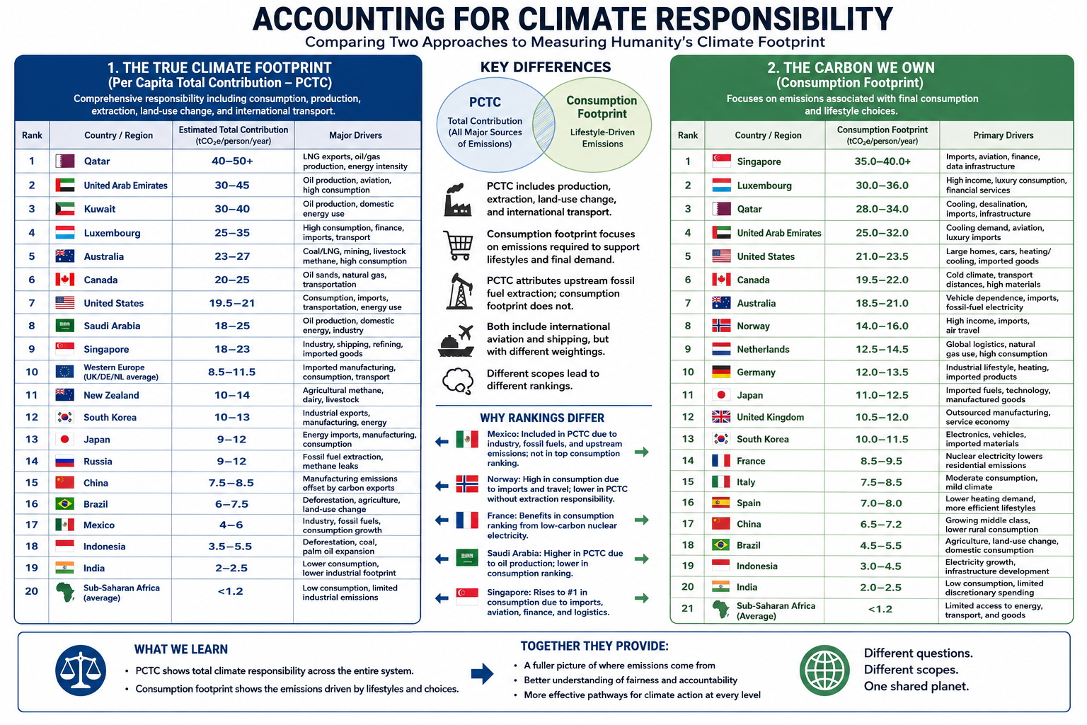
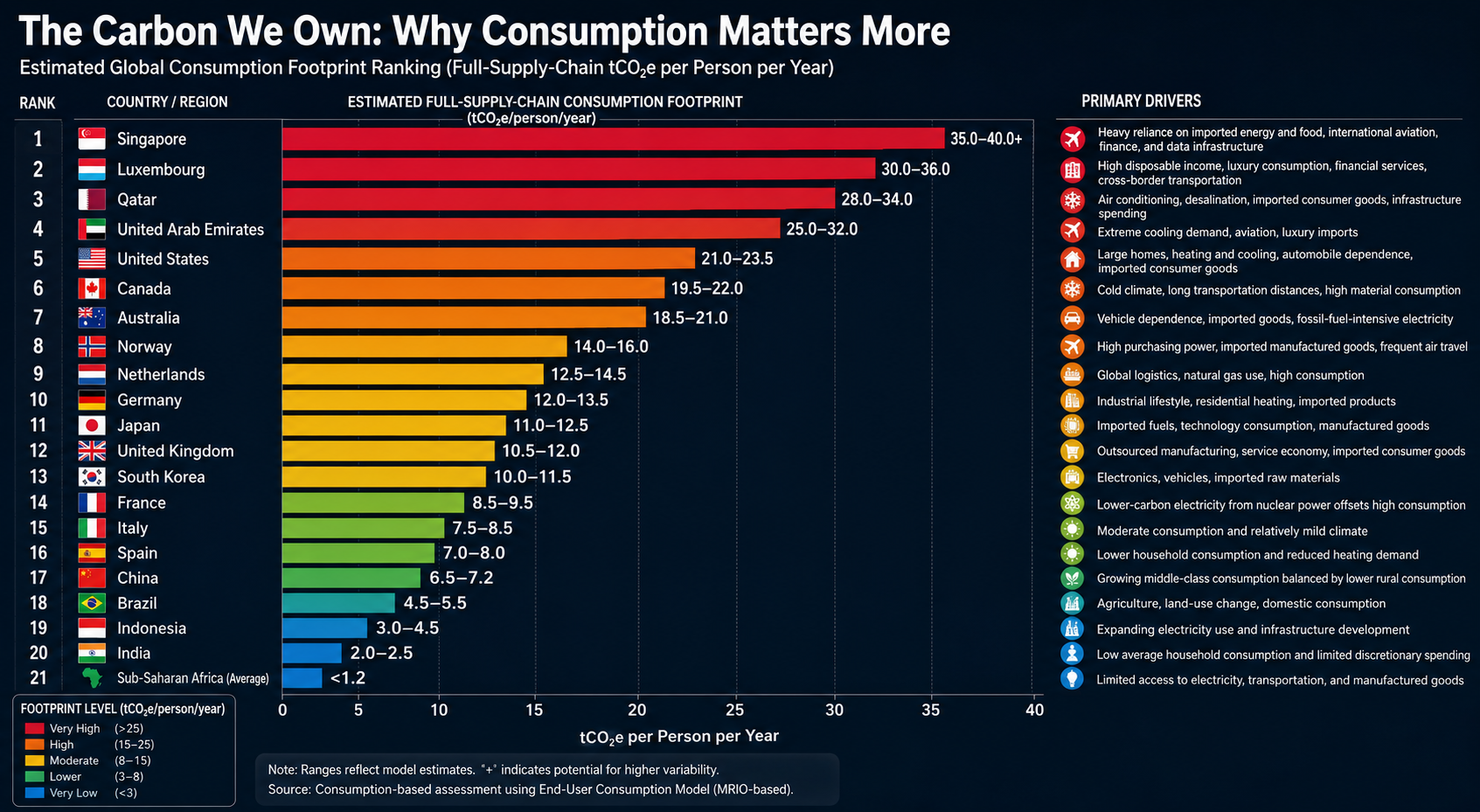
This is why consumption-based accounting provides a more accurate picture of climate responsibility than production-based accounting alone.

For example, if a smartphone is manufactured in Asia using coal-generated electricity and then shipped across the Pacific to a consumer in Los Angeles, the emissions from mining, manufacturing, transportation, and delivery are ultimately driven by the purchasing decision. Under consumption-based accounting, those emissions are attributed to the American consumer rather than solely to the country where the phone was manufactured.

Read the full explanation and view the rankings here:

http://membrane.com/global_warming/Accounting-for-Climate-Responsibility.html#the-carbon-we-own

The Production Problem

The production side of the equation is likewise influenced by self-interest and economic incentives, but it is also shaped by ideological movements that obstruct effective climate action.

Two distinct, though sometimes overlapping, ideologies are particularly important:

Denialism is characterized by the rejection of scientific evidence, refusal to engage with empirical data, and reliance on misinformation or rhetorical distraction. Its primary objective is often the protection of political, ideological, or economic interests by undermining the scientific consensus.

Ecofascism combines elements of denialism with authoritarian, exclusionary, or extremist beliefs. In its most extreme forms, it portrays environmental collapse as acceptable—or even desirable—because it is viewed as reducing populations or preserving resources for groups considered more deserving than others. This ideology has historically been associated with racist, xenophobic, or eugenicist beliefs and rejects principles of equality and shared human responsibility.

The distinction is important. Traditional denialism primarily seeks to delay or prevent climate policy. Ecofascism goes further by framing unequal human survival as an acceptable or even desirable outcome — eliminationist logic.

Why This Matters

Climate change is not simply a technological or economic challenge. It is also a question of values.

On one side, excessive consumption drives demand for fossil fuels, resource extraction, and emissions. On the other, ideologies that reject science or rationalize unequal human suffering weaken society’s ability to respond effectively to the crisis.

Both sides must be addressed if meaningful progress is to be made.

State Your Climate State

Posted on 2026/07/24 by admin

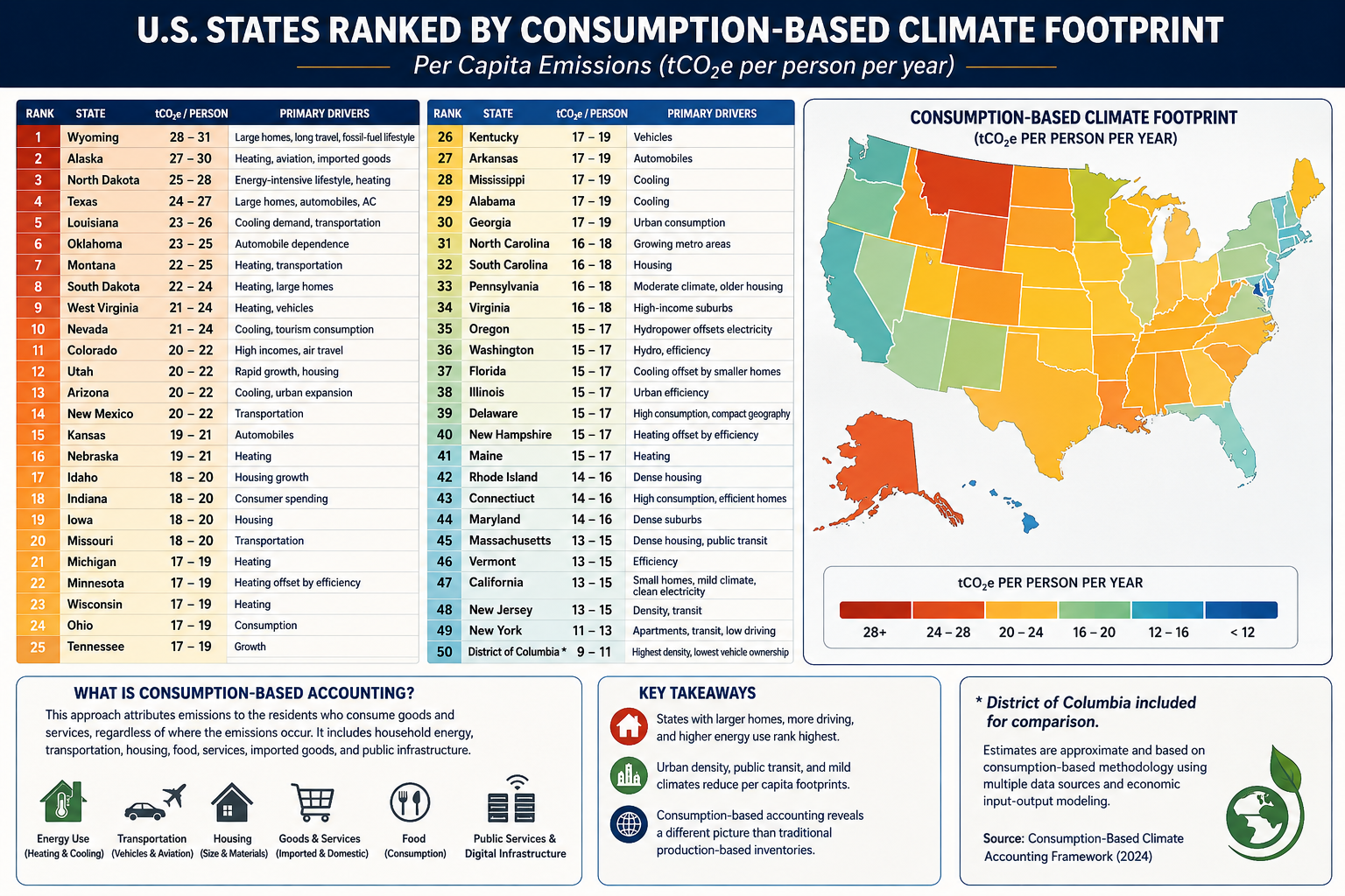
Estimated Consumption-Based Climate Footprint

(tCO₂e per person per year)

Rank	State	Estimated Footprint	Primary Drivers
1	Wyoming	28–31	Large homes, long travel distances, fossil-fuel lifestyle
2	Alaska	27–30	Heating, aviation, imported goods
3	North Dakota	25–28	Energy-intensive lifestyle, heating
4	Texas	24–27	Large homes, automobiles, air conditioning
5	Louisiana	23–26	Cooling demand, transportation
6	Oklahoma	23–25	Automobile dependence
7	Montana	22–25	Heating, transportation
8	South Dakota	22–24	Heating, large homes
9	West Virginia	21–24	Heating, vehicles
10	Nevada	21–24	Cooling, tourism consumption
11	Colorado	20–22	High incomes, air travel
12	Utah	20–22	Rapid growth, housing
13	Arizona	20–22	Cooling, urban expansion
14	New Mexico	20–22	Transportation
15	Kansas	19–21	Automobiles
16	Nebraska	19–21	Heating
17	Idaho	18–20	Housing growth
18	Indiana	18–20	Consumer spending
19	Iowa	18–20	Housing
20	Missouri	18–20	Transportation
21	Michigan	17–19	Heating
22	Minnesota	17–19	Heating offset by efficiency
23	Wisconsin	17–19	Heating
24	Ohio	17–19	Consumption
25	Tennessee	17–19	Growth
26	Kentucky	17–19	Vehicles
27	Arkansas	17–19	Automobiles
28	Mississippi	17–19	Cooling
29	Alabama	17–19	Cooling
30	Georgia	17–19	Urban consumption
31	North Carolina	16–18	Growing metro areas
32	South Carolina	16–18	Housing
33	Pennsylvania	16–18	Moderate climate, older housing
34	Virginia	16–18	High-income suburbs
35	Oregon	15–17	Hydropower offsets electricity
36	Washington	15–17	Hydro, efficiency
37	Florida	15–17	Cooling offset by small homes
38	Illinois	15–17	Urban efficiency
39	Delaware	15–17	High consumption, compact geography
40	New Hampshire	15–17	Heating offset by efficiency
41	Maine	15–17	Heating
42	Rhode Island	14–16	Dense housing
43	Connecticut	14–16	High consumption, efficient homes
44	Maryland	14–16	Dense suburbs
45	Massachusetts	13–15	Dense housing, public transit
46	Vermont	13–15	Efficiency
47	California	13–15	Small homes, mild climate, clean electricity
48	New Jersey	13–15	Density, transit
49	New York	11–13	Apartments, transit, low driving
50	District of Columbia*	9–11	Highest density, lowest vehicle ownership

(*Included for comparison.)

Accounting Method

Using the methodology from your consumption-based accounting paper, the rankings would look quite different from conventional state CO₂ inventories. Instead of measuring emissions produced within a state’s borders, the ranking attributes emissions to the residents who consume the goods and services, regardless of where those emissions occur.

The principal variables would include:

Household energy consumption
Heating and cooling demand
Transportation (vehicle ownership, VMT, aviation)
Housing size
Household income and purchasing power
Consumption of imported manufactured goods
Food consumption
Public and private services
Data center and digital infrastructure usage
Construction materials and embodied carbon

Because imported goods are attributed to consumers, states with high incomes and high levels of consumption generally rise in the rankings, while manufacturing states fall relative to production-based inventories.

What stands out?

Highest per-capita footprints

These states combine several characteristics:

Large single-family homes
Long commuting distances
High vehicle ownership
Significant heating or cooling demand
Frequent air travel
Higher embodied consumption in housing and infrastructure

Texas, Alaska, Wyoming, and North Dakota score highly not simply because of fossil-fuel production, but because residents tend to consume more energy per person.

Lowest per-capita footprints

The Northeast and California benefit from:

Smaller living spaces
Greater urban density
More public transportation
Lower vehicle miles traveled
Cleaner electricity
Higher building efficiency

New York illustrates the effect well. Although it has one of the largest economies in the world, the average resident lives in a much smaller dwelling, drives less, and relies more on mass transit than residents of most other states, resulting in one of the lowest per-capita consumption footprints.

Comparison with traditional accounting

Under conventional EPA production-based accounting:

Texas is by far the largest emitter because of industry and energy production.
California appears relatively high due to its large economy.
Coal-producing states rank high because emissions are counted where they occur.

Under consumption-based accounting, the question changes to:

“How much climate impact does the average resident’s lifestyle require?”

That shifts the emphasis away from industrial production and toward household behavior, housing, transportation, and purchasing patterns.

For an even more rigorous version suitable for publication, you could develop a state-level Multi-Regional Input-Output (MRIO) model analogous to your international consumption framework. Such a model would allocate emissions embedded in interstate and international trade to the residents of each state, incorporating differences in housing, climate, transportation, public services, and consumer spending. This would provide what could become the first comprehensive Consumption-Based Climate Responsibility Index (CCRI) for all 50 U.S. states.

The Composite Climate Responsibility Index (CCRI): A Lifecycle, Population-Normalized Framework for Measuring State-Level Climate Responsibility

Posted on 2026/07/24 by admin

by Daniel Brouse

The Composite Climate Responsibility Index (CCRI): A Lifecycle, Population-Normalized Framework for Measuring State-Level Climate Responsibility

Abstract

Greenhouse gas accounting has traditionally relied on territorial emissions—the greenhouse gases emitted within a political boundary. While this approach provides a standardized framework for national and subnational reporting, it systematically underestimates the climate responsibility of fossil fuel-producing regions by excluding upstream methane releases, fossil fuel extraction, refining, petrochemical processing, and liquefied natural gas (LNG) operations. Consequently, jurisdictions that export carbon-intensive fuels often appear to have disproportionately low climate impacts relative to the emissions they enable elsewhere.

This paper introduces the Composite Climate Responsibility Index (CCRI), a lifecycle-based, population-normalized metric that integrates direct emissions with upstream and industrial contributions to provide a more comprehensive assessment of climate responsibility. By incorporating territorial emissions, extraction activities, processing emissions, and upstream methane releases, CCRI captures the complete climate burden associated with fossil fuel production. Normalizing by population further facilitates equitable comparisons among jurisdictions of vastly different sizes.

The resulting framework reveals that many energy-exporting states possess per-capita climate burdens several times larger than those suggested by conventional inventories. CCRI offers policymakers, researchers, and the public a more representative metric for evaluating climate responsibility and designing equitable mitigation strategies.

1. Introduction

Climate policy has historically focused on territorial greenhouse gas inventories reported under the United Nations Framework Convention on Climate Change (UNFCCC). These inventories assign emissions to the jurisdiction in which they physically occur. While appropriate for international reporting, territorial accounting does not fully represent the climate impacts associated with fossil fuel production.

For example, coal mined in Wyoming may ultimately be combusted in Texas or overseas. Natural gas extracted in Pennsylvania may be liquefied in Louisiana and consumed in Europe or Asia. Existing inventories allocate combustion emissions to the point of use while largely excluding the upstream activities that make fossil fuel consumption possible.

This accounting structure creates a disconnect between production and responsibility. Fossil fuel-producing regions often exhibit relatively modest reported emissions despite facilitating substantially larger global greenhouse gas releases.

The Composite Climate Responsibility Index addresses this limitation by expanding the accounting boundary to include the entire fossil fuel production chain.

2. Conceptual Framework

Climate responsibility extends beyond smokestacks and tailpipes.

Every fossil fuel undergoes a sequence of climate-relevant processes before combustion:

Exploration
Extraction
Processing
Transportation
Storage
Distribution
Combustion

Current inventories emphasize the final stages while giving comparatively little weight to the earlier phases, despite substantial emissions from methane leakage, venting, flaring, compressor stations, refineries, LNG facilities, and petrochemical complexes.

The CCRI recognizes these emissions as integral components of fossil fuel production rather than incidental byproducts.

3. Definition of the Composite Climate Responsibility Index

The Composite Climate Responsibility Index is defined as

[
\boxed{
CCRI=
\frac{
E_{\text{territorial}}
+
E_{\text{upstream}}
+
E_{\text{processing}}
+
E_{\text{extraction}}
}
{P}
}
]

where

(E_{\text{territorial}}) represents direct greenhouse gas emissions occurring within the jurisdiction;
(E_{\text{upstream}}) represents methane leakage, venting, flaring, compressor emissions, gathering systems, and other fugitive emissions occurring prior to end-use combustion;
(E_{\text{processing}}) represents emissions associated with petroleum refining, LNG facilities, petrochemical production, natural gas processing plants, and related industrial infrastructure;
(E_{\text{extraction}}) represents emissions directly associated with coal mining, oil production, natural gas extraction, drilling, pumping, and associated operations;
(P) represents the jurisdiction’s population.

The resulting metric is expressed as

metric tons CO₂-equivalent per capita per year.

4. Advantages Over Traditional Inventories

Traditional greenhouse gas inventories answer the question:

“How much greenhouse gas is emitted inside this state?”

CCRI instead asks:

“How much climate forcing is generated because this state produces fossil fuels?”

This distinction fundamentally changes state rankings.

Large population centers often dominate territorial emissions because of transportation and electricity demand.

However, production-based accounting reveals that relatively small states can exert disproportionately large global climate impacts through fossil fuel extraction and processing.

5. Components of the Index

5.1 Territorial Emissions

These include all greenhouse gases released within state boundaries, including

electricity generation
transportation
industrial processes
residential and commercial energy use
agriculture
waste management

These values are generally available through EPA greenhouse gas inventories.

5.2 Upstream Emissions

Upstream emissions include

methane leakage
venting
flaring
abandoned wells
gathering pipelines
compressor stations
storage facilities

Methane is particularly important because its near-term warming potential greatly exceeds that of carbon dioxide.

Failure to include upstream methane significantly underestimates the climate burden of natural gas production.

5.3 Processing Emissions

Processing emissions include

oil refining
LNG liquefaction
petrochemical production
fertilizer manufacturing
hydrogen production from fossil fuels
natural gas processing

Many refining states emit relatively modest territorial greenhouse gases compared with the enormous climate impacts associated with processing fossil fuels destined for global markets.

5.4 Extraction Emissions

Extraction includes

coal mining
drilling operations
hydraulic fracturing
pumping
mining equipment
dewatering
mine methane
associated infrastructure

Coal-producing regions often exhibit exceptionally large extraction-related emissions.

6. Why Population Matters

Absolute emissions measure scale.

Per-capita emissions measure responsibility.

Population normalization allows meaningful comparisons between states of vastly different sizes.

For example, Texas produces the largest absolute climate burden in the United States because of its enormous oil, gas, refining, petrochemical, and power sectors.

Conversely, Wyoming’s small population means that its production-related emissions translate into one of the highest per-capita climate burdens in the world.

Thus, CCRI distinguishes between total contribution and individual responsibility.

7. Policy Applications

CCRI provides policymakers with several advantages.

It can

identify regions with disproportionate upstream emissions;
improve methane reduction strategies;
prioritize investments in emissions monitoring;
support equitable climate policy;
inform carbon pricing mechanisms;
evaluate fossil fuel subsidies;
guide transition assistance for energy-producing regions;
improve state-to-state comparisons.

Because CCRI incorporates lifecycle emissions, it aligns more closely with the physical drivers of climate change than territorial inventories alone.

8. Illustrative Results

Applying the framework to U.S. states suggests that fossil fuel-producing regions dominate per-capita climate responsibility.

Illustrative rankings include:

Wyoming
North Dakota
West Virginia
New Mexico
Louisiana
Alaska
Oklahoma
Texas
Pennsylvania
Kentucky

These rankings differ substantially from traditional greenhouse gas inventories, which are dominated by population size rather than fossil fuel production.

9. Limitations

Like all composite indicators, CCRI depends on the quality of underlying datasets.

Future refinements should incorporate

satellite methane observations,
lifecycle emission factors,
temporal variability,
exported fossil fuel carbon content,
uncertainty analysis,
probabilistic confidence intervals.

Additional weighting schemes may also be developed to distinguish short-lived climate pollutants from long-lived greenhouse gases.

10. Conclusion

The Composite Climate Responsibility Index represents a significant advancement in greenhouse gas accounting by extending responsibility beyond territorial emissions to encompass the complete fossil fuel production chain. It recognizes that extraction, processing, and upstream methane emissions are not peripheral activities but essential components of the carbon economy.

By integrating these sources and normalizing by population, CCRI offers a more comprehensive measure of climate responsibility than traditional inventories. It reveals that many jurisdictions with modest reported emissions play an outsized role in enabling global fossil fuel consumption, while densely populated states often appear less carbon-intensive when viewed through a production-based lens.

As climate policy evolves toward lifecycle accounting and supply-side mitigation, the Composite Climate Responsibility Index provides a transparent, scalable, and scientifically grounded framework for evaluating the true climate burden associated with fossil fuel production. It complements existing territorial inventories rather than replacing them, offering decision-makers a broader perspective on responsibility, equity, and the pathways toward effective emissions reduction.

America’s New Tariff Landscape: Who Gets Taxed—and Who Really Pays?

Posted on 2026/07/24 by admin

Introduction

The latest U.S. tariff framework is now in place, and while tariffs are collected at the border, it’s American families who ultimately pay most of the bill.

📊 Highlights:
• Average household: +$2,000–$2,700 per year
• Buying a new home and a new car? The added cost from tariffs on steel, aluminum, lumber, vehicles, appliances, and other goods could exceed $30,000–$50,000.
• New tariffs now cover nearly 99.4% of U.S. imports from 60 trading partners, while additional 50% tariffs on many Canadian products are scheduled to begin in August.

The article explains what changed, which goods are affected, who legally pays the tariff, and who ultimately bears the economic burden.

Read the full analysis and decide for yourself: Are tariffs protecting American industry, or are they becoming one of the largest hidden taxes on American consumers?

1. Newly Enacted Tariffs: Section 301 Forced Labor Framework

Effective July 24, 2026, the United States implemented a new tariff regime targeting imports from approximately 60 trading partners, representing 99.4% of all U.S. imports. The tariffs are based on supply-chain forced labor investigations.

Tariff Rates

10% Base Rate
- Canada
- Mexico
- United Kingdom
- India
- Argentina
10%–12.5% Blended Rate
- European Union
- Japan
- South Korea
- Taiwan
12.5% Flat Rate
- China
- Vietnam
- Australia
- Singapore
- 34 additional economies under investigation

Exemptions

Several strategically important commodities remain exempt, including:

Crude oil
Natural gas
Fertilizer
Selected primary food products

These tariffs also do not stack with existing Section 232 national security duties.

2. Upcoming Canadian Tariffs: Section 338

Beginning August 19, 2026, the United States is scheduled to impose 50% retaliatory tariffs on approximately $20 billion of Canadian imports under Section 338 of the Tariff Act of 1930.

Products Subject to the 50% Tariff

Dairy products
Wine and other alcoholic beverages
Automobiles
Auto parts
Cement
Hockey equipment
Plywood
Particleboard
Paper products
Clothing
Furniture

These tariffs bypass normal CUSMA (USMCA) preferential treatment.

Exemptions

The following Canadian exports are excluded:

Energy products
Potash
Fish
Critical minerals

3. Existing Tariffs That Remain in Effect

Several major tariff programs adopted during 2025 and 2026 continue unchanged.

Section 232 National Security Tariffs

These duties continue to apply to steel and aluminum imports, including tariffs reaching 50% on certain Canadian steel and aluminum products.

Existing Canadian Import Tariffs

Additional tariffs remain in place on:

25% on non-CUSMA-compliant auto parts
25% on upholstered furniture and kitchen cabinets
10% tariff on Canadian softwood lumber, with combined anti-dumping and countervailing duties pushing the effective rate to approximately 45%

Section 301 China Tariffs

Long-standing tariffs on Chinese imports also remain active, with rates reaching 25% on numerous products, including:

Industrial machinery
Technology equipment
Electronic components
Strategic manufacturing inputs

Current U.S. Tariff Framework

Tariff Program	Primary Target	Rate	Status
Section 301 – Forced Labor	60 trading partners	10%–12.5%	Active (July 24, 2026)
Section 338 – Canada	Autos, dairy, wine, cement, consumer goods	50%	Begins August 19, 2026
Section 232 – National Security	Steel & aluminum	25%–50%	Active
Section 301 – China	Industrial & technology products	Up to 25%	Active

Who Really Pays Tariffs?

Legally, tariffs are paid by the U.S. importer when goods enter the country through Customs and Border Protection.

Economically, however, that is only the beginning of the story.

Importers generally recover those additional costs by increasing the prices they charge wholesalers, retailers, manufacturers, and ultimately consumers. Numerous economic studies of recent U.S. tariffs have found that most of the cost is passed through to American businesses and households rather than absorbed by foreign exporters.

In some industries, foreign suppliers may reduce prices to remain competitive, meaning they share part of the burden. But the overall trade data and pricing evidence show that the majority of tariff costs are ultimately borne within the United States through higher prices, reduced business margins, or both.

In other words, while tariffs are collected at the border from importers, they function much like a domestic consumption tax. The final bill is usually paid by American businesses and consumers—not by foreign governments.

Conclusion

For the average American household, the new tariff regime is expected to increase costs by approximately $2,000–$2,700 per year. For families purchasing a newly built home and a new vehicle, the cumulative tariff burden can easily exceed $30,000–$50,000 through higher prices on construction materials, automobiles, appliances, and other imported goods. While tariffs are collected at the border from importers, they are ultimately borne by American businesses and consumers in the form of higher prices—a tax paid not to foreign governments, but by U.S. households.

Accounting for Climate Responsibility

Posted on 2026/07/23 by admin

by Daniel Brouse

Comparing Two Approaches to Measuring Humanity’s Climate Footprint

Climate responsibility depends on how emissions are assigned. Traditional territorial accounting attributes emissions to the country where they occur, but globalization has made that approach increasingly incomplete. Modern supply chains, international trade, and service-based economies often separate where emissions are produced from who ultimately benefits from them.

To explore this problem from two different perspectives, I developed two complementary accounting frameworks.

The first paper, The True Climate Footprint: Measuring Per Capita Total Contribution Beyond Territorial Emissions, introduces the Per Capita Total Contribution (PCTC) framework. PCTC seeks to estimate an individual’s or nation’s complete climate responsibility by incorporating not only consumption, but also several major sources of emissions that are frequently omitted from conventional carbon accounting.

The True Climate Footprint: Measuring Per Capita Total Contribution

The PCTC framework includes:

Consumption-based emissions
Land-use change and deforestation
Upstream fossil fuel extraction (methane leakage, flaring, and coal mine emissions)
International aviation and maritime shipping
All major greenhouse gases (CO₂, CH₄, N₂O, and others expressed as CO₂-equivalent)
Responsibility associated with fossil fuel production where appropriate

The second paper, The Carbon We Own: Why Consumption Matters More, examines climate responsibility from a different perspective. Rather than estimating total climate contribution, it focuses specifically on the carbon footprint required to support modern lifestyles using a consumption-based accounting approach.

The Carbon We Own: Why Consumption Matters More

This framework emphasizes:

Multi-Regional Input-Output (MRIO) accounting
Direct household energy use
Embedded emissions in imported goods
Public and private services
Lifestyle and purchasing choices

Unlike PCTC, this framework intentionally places less emphasis on fossil fuel extraction and producer responsibility in order to better isolate the climate impacts associated with everyday consumption.

After completing the first paper, I wanted to examine the climate footprint from the perspective of the consumer rather than the entire climate system. The PCTC framework provides a comprehensive measure of total responsibility, but it does not distinguish as clearly between emissions driven by individual lifestyle choices and those associated with resource extraction or national production.

A consumption-based framework highlights decisions that individuals and societies can influence more directly. Choices such as lowering a home’s thermostat, improving insulation, selecting public transportation or electric vehicles instead of internal combustion vehicles, reducing air travel, or purchasing fewer carbon-intensive goods become more visible within the accounting. It also better captures the increasingly important role of service-based economies. While services may appear less energy-intensive than manufacturing, sectors such as healthcare, finance, telecommunications, cloud computing, and artificial intelligence rely on extensive digital infrastructure—including energy-hungry data centers—that can be substantially underrepresented in traditional emissions inventories.

Finally, I wanted a more detailed comparison among developed economies, particularly within Europe. Countries such as Norway and France illustrate why accounting methodology matters. Norway has one of the world’s cleanest domestic electricity systems, powered primarily by hydropower, yet it is also a major exporter of oil and natural gas. France, by contrast, derives much of its electricity from nuclear power, resulting in comparatively low-carbon domestic energy while maintaining a high standard of living. Comparing these countries under both frameworks reveals how different accounting methods assign responsibility and helps illustrate the strengths and limitations of each approach.

Taken together, these two papers do not compete—they answer different questions. Per Capita Total Contribution (PCTC) asks, What is humanity’s full climate responsibility? Consumption-based accounting asks, What emissions are required to sustain the lifestyle of the average resident? Used together, they provide a more complete understanding of climate responsibility than either framework alone.

Conclusion

Although The True Climate Footprint and The Carbon We Own both seek to improve upon traditional territorial emissions accounting, they answer different questions because they are built on different accounting frameworks.

The True Climate Footprint uses the Per Capita Total Contribution (PCTC) framework to estimate an individual’s or nation’s complete contribution to climate change. It extends beyond consumption to include land-use change, upstream fossil fuel extraction, international shipping and aviation, and the full spectrum of greenhouse gases. In some cases, it also attributes responsibility associated with fossil-fuel production, providing a broad measure of humanity’s total climate impact.

By contrast, The Carbon We Own focuses specifically on consumption-based climate responsibility. Using Multi-Regional Input-Output (MRIO) accounting, it assigns emissions to the final consumer by emphasizing direct household energy use, embedded emissions in imported goods, services, and lifestyle choices. It intentionally deemphasizes extraction and producer responsibility in order to better represent the carbon footprint required to sustain modern patterns of consumption.

Because these frameworks measure different aspects of climate responsibility, their rankings are not expected to be identical.

Mexico provides a useful illustration. Under the PCTC framework, Mexico’s estimated footprint includes domestic industry, fossil fuel production, growing consumption, and upstream emissions, resulting in an estimated contribution of approximately 4–6 tonnes of CO₂-equivalent per person per year. In the consumption-based analysis, however, Mexico does not appear among the highest-ranking countries because the focus is limited to end-user consumption, and the published rankings emphasize the world’s largest per-capita consumption footprints.

Similar differences appear elsewhere. Norway’s position changes substantially because one framework incorporates the climate responsibility associated with fossil fuel production, while the other emphasizes domestic consumption. France benefits in the consumption-based analysis because its low-carbon nuclear electricity reduces household emissions despite maintaining a high standard of living. Saudi Arabia ranks differently depending on whether responsibility is assigned to oil production or to energy consumption. Singapore rises dramatically under consumption accounting because imported goods, international aviation, finance, logistics, and digital infrastructure contribute heavily to its consumption footprint despite relatively limited domestic manufacturing.

These examples demonstrate that accounting methodology influences how climate responsibility is distributed. Production-based, consumption-based, and total-contribution frameworks each illuminate different dimensions of the global climate system.

Rather than viewing these approaches as competing methodologies, they should be regarded as complementary analytical tools. The Per Capita Total Contribution (PCTC) framework asks, What is a nation’s or individual’s total contribution to climate change? The consumption-based framework asks, What emissions are required to sustain the average resident’s lifestyle? Together, they provide a more complete understanding of climate responsibility than either approach can achieve alone, revealing both the systemic impacts of resource production and the powerful role of consumer demand in shaping the global climate.

The Carbon We Own: Why Consumption Matters More

Posted on 2026/07/222026/07/23 by admin

by Daniel Brouse

For decades, climate responsibility has often been measured by where fossil fuels are extracted or where products are manufactured. While useful for tracking national emissions, this production-based approach can misrepresent who ultimately drives demand.

A consumption-based accounting approach shifts the focus to the end user. Instead of assigning emissions to the country where a product is made, it attributes emissions to the people and businesses that ultimately consume the energy, goods, and services.

Under this framework, every kilowatt-hour of electricity, every heating bill, every medical service, and every consumer product is assigned to its final destination.

For example, if a smartphone is manufactured in Asia using electricity generated from coal and then shipped across the Pacific to a consumer in Los Angeles, the emissions associated with mining, manufacturing, transportation, and delivery are attributed to the American consumer—not the manufacturing country.

This approach provides a more accurate picture of the carbon footprint associated with modern lifestyles.

How Consumption-Based Carbon Accounting Works

Most consumption analyses rely on Multi-Regional Input-Output (MRIO) economic models, which trace emissions through global supply chains before assigning them to final consumers.

Individual carbon footprints are generally divided into three major categories:

1. Direct Household Energy

Emissions from energy used directly by households, including:

Home heating and cooling
Residential electricity
Personal vehicle fuel
Digital activities such as internet usage and streaming services

2. Embedded Goods

Emissions generated while producing and transporting purchased products, including:

Electronics
Vehicles
Furniture
Clothing
Building materials
Household appliances

These emissions often occur in countries far from the final consumer.

3. Services

Many of the largest emissions in developed economies come not from physical products but from services, including:

Healthcare
Commercial aviation
Banking and finance
Cloud computing
Water and wastewater treatment
Telecommunications

In the United States alone, healthcare contributes roughly 1.6 tonnes of CO₂-equivalent emissions per person each year, illustrating how service-based economies can generate substantial carbon footprints even as heavy industry declines.

Major Findings from Global Consumption Accounting

The Rise of Service Economies

In wealthy economies such as Singapore, Luxembourg, and several Western European countries, manufacturing represents only a small portion of domestic emissions.

Instead, much of their climate impact comes from:

Commercial aviation
Financial systems
Cloud computing
Global logistics
Luxury consumption
High levels of imported goods

As economies become increasingly service-oriented, carbon emissions become embedded in complex international supply chains rather than local smokestacks.

Geography Still Matters

Climate strongly influences direct household energy use.

Countries with long, cold winters or extremely hot summers require substantially more energy for climate control.

For example:

Canada and the United States consume large amounts of energy for winter heating and summer air conditioning, particularly because of larger average home sizes.
Australia records comparatively higher emissions from agriculture, mining, and infrastructure development than from residential heating.

Local climate remains an important contributor even after imported goods are included.

China’s Manufacturing Versus Consumption

China illustrates one of the largest differences between production-based and consumption-based accounting.

Because China manufactures enormous quantities of products for export, its territorial emissions are among the highest in the world.

However, when emissions are allocated to the people who ultimately purchase those products, China’s domestic per-capita consumption footprint is estimated at roughly 6.8 tonnes of CO₂-equivalent per year.

This highlights the distinction between:

Production emissions (where goods are made)
Consumption emissions (who ultimately benefits from those goods)

Many products manufactured in China are consumed in North America and Europe, meaning a significant share of manufacturing emissions is driven by foreign demand.

Consumption Footprints Across Europe

Norway: Clean Electricity, High Consumption

Estimated consumption footprint: 14.8 tonnes CO₂e per person

Norway’s electricity is more than 85% hydropower, giving it one of the cleanest electrical grids in the world.

Yet Norwegians have high purchasing power and consume large quantities of imported goods, including:

Electric vehicles
Consumer electronics
Luxury goods
Imported foods

Norway also has one of the world’s highest rates of air travel per capita, increasing its service-sector emissions.

The result is a consumption footprint considerably larger than its territorial emissions suggest.

United Kingdom: Outsourcing Manufacturing

Estimated consumption footprint: 11.2 tonnes CO₂e per person

The United Kingdom has significantly reduced domestic production emissions by retiring coal-fired power plants and expanding renewable electricity.

However, much of the country’s manufacturing has shifted overseas.

The UK imports large quantities of:

Electronics
Machinery
Clothing
Construction materials

Consequently, much of its carbon footprint exists outside its borders, while domestic emissions increasingly come from finance, digital infrastructure, commercial services, and transportation.

France: The Nuclear Advantage

Estimated consumption footprint: 9.2 tonnes CO₂e per person

France demonstrates how a low-carbon electricity system can substantially reduce consumption emissions.

French households enjoy living standards comparable to neighboring Western European countries, yet much of their residential electricity, rail transportation, and heating is supplied by nuclear energy.

As a result, France’s direct household energy emissions are estimated to be roughly 30% lower than those of many neighboring countries with similar consumption patterns.

China Compared with Western Europe

When emissions are assigned to consumers rather than producers, an average citizen in countries such as Germany or the United Kingdom is responsible for nearly twice the carbon footprint of the average Chinese citizen.

Although China’s middle class continues to grow and domestic consumption is increasing, much of the country’s industrial output still serves international markets.

This comparison illustrates a key insight of consumption-based accounting:

A nation’s production does not necessarily reflect the climate impact of its residents’ lifestyles.

A Different Way to Think About Climate Responsibility

Consumption-based accounting reframes climate responsibility by asking a simple question:

Who ultimately benefits from the energy and resources consumed?

Rather than focusing solely on where emissions occur, this approach follows products and services through global supply chains to their final users.

For affluent economies that import large volumes of manufactured goods while exporting much of their industrial production, consumption-based accounting often reveals substantially higher per-capita climate footprints than traditional territorial inventories.

Viewed through this lens, lifestyle choices, purchasing power, housing, transportation, travel, healthcare, digital services, and overall consumption patterns become the primary drivers of individual climate responsibility.

Ultimately, the atmosphere responds to total emissions, regardless of where they occur. Consumption-based accounting provides a complementary perspective to traditional production-based inventories by connecting those emissions to the people and economies whose demand created them.

Global Consumption Footprint Rankings

Traditional emissions inventories assign carbon pollution to the country where fossil fuels are extracted or products are manufactured. A consumption-based accounting approach instead assigns those emissions to the people and economies that ultimately consume the goods and services.

The rankings below are based on an End-User Consumption Model, which allocates the full upstream supply-chain emissions—including raw material extraction, manufacturing, international transportation, agricultural land-use change, and other embedded emissions—to the final purchaser.

Rather than measuring where emissions occur, this framework estimates the carbon footprint required to sustain the average lifestyle of a country’s residents. It reflects direct household energy use, consumption of imported goods, transportation, public infrastructure, and carbon-intensive services.

Estimated Global Consumption Footprint Ranking

Rank	Country / Region	Estimated Full-Supply-Chain Consumption Footprint (tCO₂e/person/year)	Primary Drivers
1	🇸🇬 Singapore	35.0–40.0+	Heavy reliance on imported energy and food, international aviation, finance, and data infrastructure
2	🇱🇺 Luxembourg	30.0–36.0	High disposable income, luxury consumption, financial services, cross-border transportation
3	🇶🇦 Qatar	28.0–34.0	Air conditioning, desalination, imported consumer goods, infrastructure spending
4	🇦🇪 United Arab Emirates	25.0–32.0	Extreme cooling demand, aviation, luxury imports
5	🇺🇸 United States	21.0–23.5	Large homes, heating and cooling, automobile dependence, imported consumer goods
6	🇨🇦 Canada	19.5–22.0	Cold climate, long transportation distances, high material consumption
7	🇦🇺 Australia	18.5–21.0	Vehicle dependence, imported goods, fossil-fuel-intensive electricity
8	🇳🇴 Norway	14.0–16.0	High purchasing power, imported manufactured goods, frequent air travel
9	🇳🇱 Netherlands	12.5–14.5	Global logistics, natural gas use, high consumption
10	🇩🇪 Germany	12.0–13.5	Industrial lifestyle, residential heating, imported products
11	🇯🇵 Japan	11.0–12.5	Imported fuels, technology consumption, manufactured goods
12	🇬🇧 United Kingdom	10.5–12.0	Outsourced manufacturing, service economy, imported consumer goods
13	🇰🇷 South Korea	10.0–11.5	Electronics, vehicles, imported raw materials
14	🇫🇷 France	8.5–9.5	Lower-carbon electricity from nuclear power offsets high consumption
15	🇮🇹 Italy	7.5–8.5	Moderate consumption and relatively mild climate
16	🇪🇸 Spain	7.0–8.0	Lower household consumption and reduced heating demand
17	🇨🇳 China	6.5–7.2	Growing middle-class consumption balanced by lower rural consumption
18	🇧🇷 Brazil	4.5–5.5	Agriculture, land-use change, domestic consumption
19	🇮🇩 Indonesia	3.0–4.5	Expanding electricity use and infrastructure development
20	🇮🇳 India	2.0–2.5	Low average household consumption and limited discretionary spending
21	Sub-Saharan Africa (Average)	<1.2	Limited access to electricity, transportation, and manufactured goods

Key Patterns

Small, Wealthy Nations Have the Largest Per-Capita Footprints

Singapore and Luxembourg rank highest despite having relatively little domestic heavy industry. Their residents consume large quantities of imported goods and services, while extensive international transportation, finance, aviation, and digital infrastructure contribute substantial embedded emissions.

High-Income, Car-Oriented Economies Form the Next Tier

The United States, Canada, and Australia consistently rank among the world’s largest per-capita consumers. Large homes, automobile-dependent communities, extensive heating or cooling needs, and high levels of discretionary consumption combine to produce substantial lifestyle-related emissions.

Low-Carbon Electricity Helps—but Doesn’t Eliminate Consumption Emissions

Countries such as France and Norway demonstrate that cleaner electricity significantly lowers household energy emissions. However, imported goods, international travel, and service-sector activities remain important contributors to their overall consumption footprints.

Manufacturing Countries Are Not Necessarily the Largest Consumers

China’s production-based emissions are among the highest globally because it manufactures goods for international markets. Under a consumption-based framework, however, the average Chinese citizen’s lifestyle footprint remains considerably lower than that of residents in many affluent Western countries.

Consumption Capacity Is the Strongest Predictor

Perhaps the clearest finding is the enormous gap between affluent economies and developing regions. Average per-capita consumption in Sub-Saharan Africa remains a small fraction of that in the world’s wealthiest nations, reflecting differences in income, energy access, transportation, housing, and consumer purchasing power.

This comparison underscores a central conclusion of consumption-based accounting: the carbon footprint of an individual is driven primarily by the scale and complexity of the lifestyle they support, rather than the geographic location where the associated emissions physically occur.