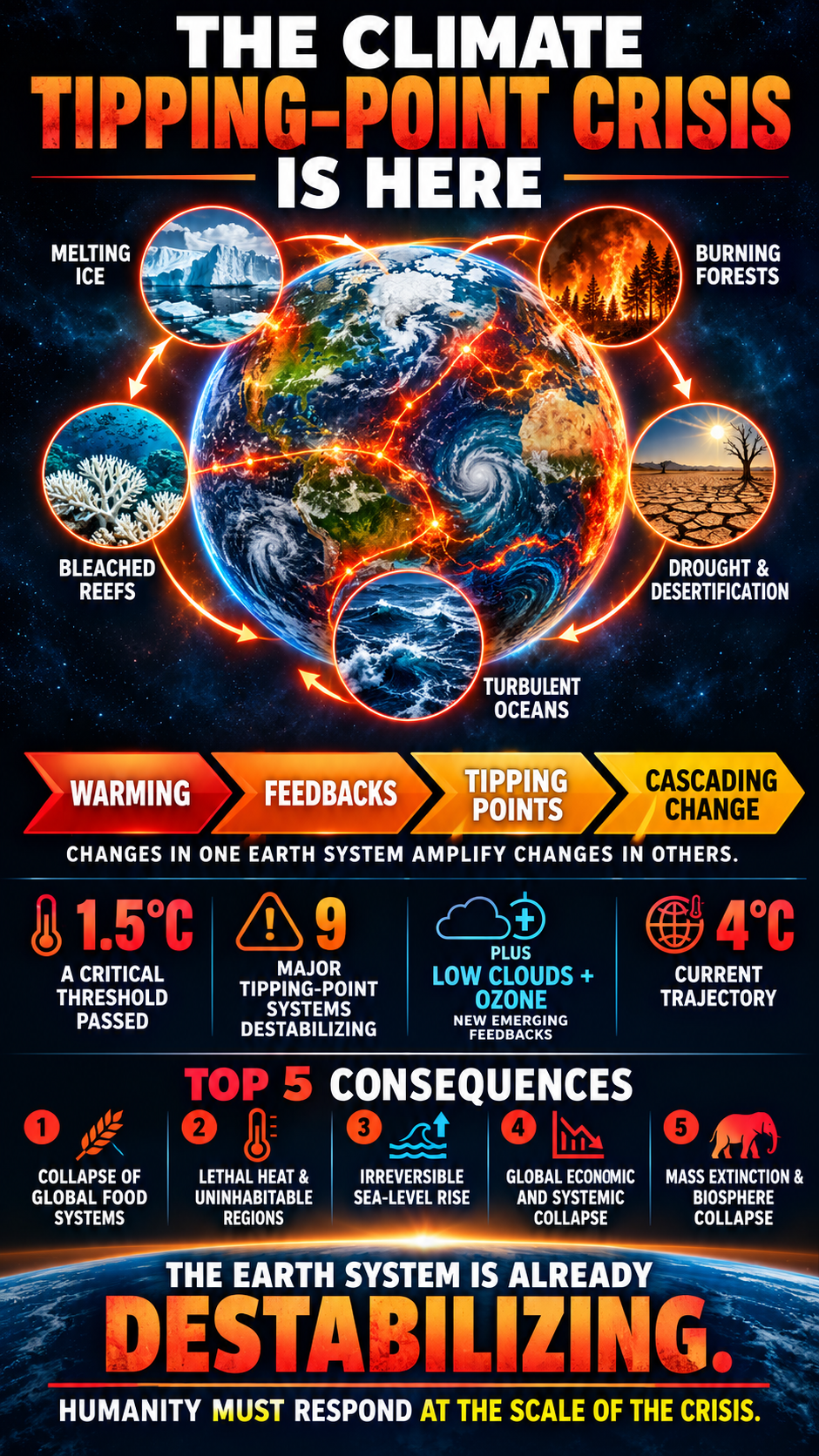
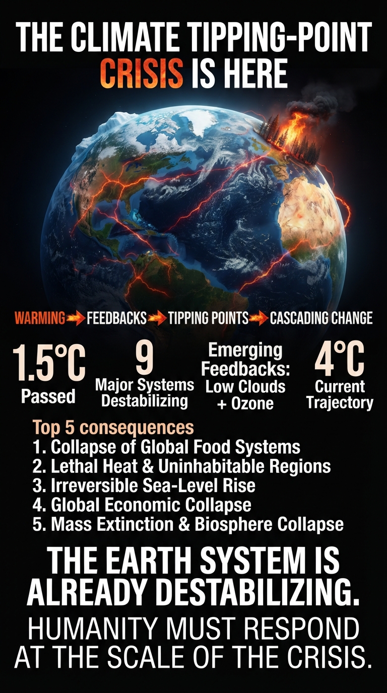
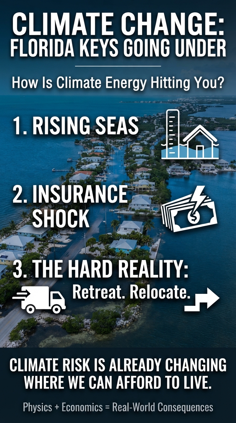
Warmest October on Record — 2026 Virtually Certain to Exceed 1.5°C
The 1.5°C threshold represents a critical point in the activation, coupling, and amplification of climate feedbacks. We have already observed the predicted outcomes. Now, the global temperature data is catching up with what the accelerating climate system has been telling us.
2026 is now virtually certain to exceed 1.5°C above pre-industrial levels, becoming only the second calendar year to cross that threshold after 2024. This prediction is based on ERA5 temperature data through October. 2026 is also most likely to become the second-warmest year on record, with approximately a 20% chance of tying or exceeding 2024, currently the warmest year on record.
Even more significant, the four-year average global temperature for 2023–2026 is also expected to exceed 1.5°C above pre-industrial levels.
These findings come from the Copernicus Climate Change Service (C3S), implemented by the European Centre for Medium-Range Weather Forecasts (ECMWF).
This is no longer simply a projection of future warming. We are observing the consequences of an increasingly interconnected climate feedback system in real time.
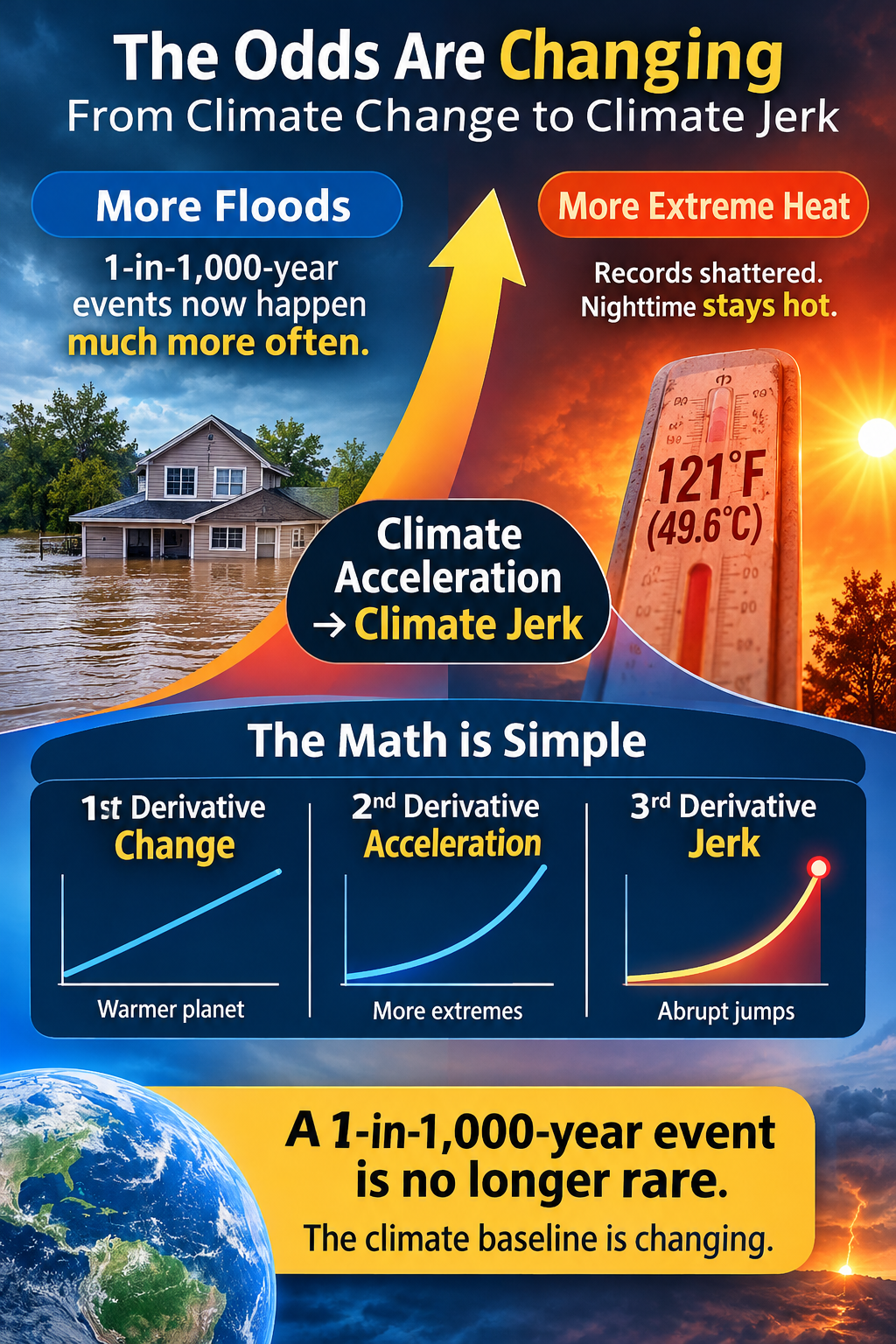
1-in-1,000-year weather events are no longer as rare as their name suggests.
Historic rainfall. Record-breaking heat. Flash droughts. Extreme storms. These events are increasingly challenging the assumptions built into historical weather records.
Why?
Because the climate baseline is changing — and so are the odds.
A 1-in-1,000-year event is not a permanent characteristic of the weather. It is a probability calculated from a particular climate distribution. Change the climate distribution, and you change the odds.
🔥 Extreme heat intensifies. 🌧️ Heavy rainfall becomes more dangerous. 🌊 Flood risks escalate. 🌾 Drought and soil-moisture feedbacks amplify heat. ⚡ Climate impacts increasingly interact and compound.
This is more than climate change. It is climate acceleration: a changing system in which warming activates feedbacks, feedbacks amplify warming, and interconnected impacts reshape the risks we face.
The question is no longer whether historical weather patterns are changing. It is whether our infrastructure, economies, insurance systems, and communities are adapting to the new probabilities.
THE ODDS ARE CHANGING. Our understanding of risk must change with them.
Introduction: When 1,000-Year Disasters Become Routine
The frequency, intensity, and clustering of so-called “1-in-1,000-year” disasters have changed dramatically since the 1990s. Events once considered exceptionally rare are now occurring repeatedly, sometimes within weeks or even days of one another.
But there is a fundamental mathematical misunderstanding behind the way these events are commonly described.
A 1-in-1,000-year event does not mean a disaster happens only once every millennium. It describes a 0.1% annual probability calculated from a particular historical climate distribution.
When the climate baseline changes, the probability distribution changes.When the distribution changes, the odds change.
A rainfall event that historically had a 0.1% annual probability can become a 1%, 2%, 4%, or even higher annual probability under substantially different climate conditions.
The event itself has not changed its statistical label. The climate conditions underlying that label have changed.
This is the critical distinction: A 1-in-1,000-year disaster is not inherently a 1-in-1,000-year event. It is a 1-in-1,000-year event under a particular set of historical conditions.
Human-caused climate change is fundamentally altering those conditions. Historical probability estimates are becoming increasingly disconnected from actual and future climate risks.
And this transformation is not limited to rainfall and flooding. Extreme heat is revealing another dimension of the same problem, with temperature extremes, soil moisture, ocean heat, and atmospheric feedbacks producing increasingly disruptive consequences.
The historical odds are changing because the underlying climate system is changing.
1. Massive Increase in Climate-Related Disasters
Data tracking extreme weather disasters show a substantial upward trajectory since the end of the 20th century.
According to data published by Yale Environment 360, climate-related disasters increased by 83% when comparing the 1980–1999 period with the subsequent 20 years.
Within that increase:
Major flood events more than doubled worldwide.
Severe storms increased by approximately 40%.
Extreme weather disasters became increasingly frequent and costly.
This is not simply a matter of experiencing more bad weather. It reflects a changing climate system in which the conditions supporting extreme events are becoming increasingly pronounced.
2. The Clustering of 1,000-Year Disasters
One of the most striking developments is the clustering of extreme precipitation events.
In the 1990s, a 1-in-1,000-year rainfall event was an exceptionally isolated occurrence. Today, multiple events of comparable historical statistical magnitude are appearing within remarkably short periods.
The 2022 Cluster
During a single five-week period in the summer of 2022, the United States experienced five separate rainfall events described as 1-in-1,000-year events:
St. Louis, Missouri
Eastern Kentucky
Southeastern Illinois
Death Valley, California
Dallas, Texas
The 2025 Cluster
During a single week in July 2025, four separate 1-in-1,000-year rainfall events struck:
Texas
North Carolina
New Mexico
Illinois
These clusters demonstrate why historical return-period statistics can no longer be interpreted as though extreme events occur independently against an unchanging climate baseline.
There is an important statistical distinction: multiple events described using historical return periods do not necessarily retain those same probabilities under today’s climate. Nor does the occurrence of several events by itself establish that they were statistically independent.
The essential point is that the historical probability distribution is changing, and the old return-period labels no longer reliably describe present-day risk.
3. The Sharp Rise in Extreme Daily Rainfall
The underlying driver of many catastrophic floods is the increasing intensity of individual precipitation events.
The U.S. Environmental Protection Agency (EPA) reports that the prevalence of extreme single-day precipitation events remained relatively steady from 1910 through the 1980s, but increased substantially beginning around 1990.
In fact, nine of the ten years with the highest extreme one-day precipitation in U.S. history have occurred since 1990.
This is particularly significant because extreme rainfall can overwhelm drainage systems, culverts, stormwater infrastructure, rivers, and flood-control structures in a matter of hours.
The problem is not simply that it rains more. The intensity of individual rainfall events is changing, pushing infrastructure beyond the conditions for which it was designed.
4. The Mathematics of Changing Return Periods: The Odds Are Changing
This is arguably the most important mathematical consequence of climate change.
A 1-in-1,000-year event is not a fixed characteristic of a rainfall event. It is a statistical probability derived from a historical climate distribution.
The return period describes the probability of an event occurring under specified climate conditions. It does not guarantee how frequently that event will occur as those conditions change.
The mathematics is straightforward:
Historical Return Period
Annual Probability
1-in-1,000 years
0.1%
1-in-500 years
0.2%
1-in-100 years
1%
1-in-50 years
2%
1-in-25 years
4%
1-in-10 years
10%
These probabilities are calculated from a particular statistical distribution. They are not permanent.
If warming increases atmospheric moisture, changes precipitation intensity, and alters storm behavior, the probability distribution shifts.
An event that previously had a 0.1% annual probability might now have a 4% annual probability.
That is a change from a nominal 1,000-year return period to a 25-year return period.
The storm does not need to become 40 times larger. Its probability of occurring at that intensity needs to increase 40-fold.
This is the fundamental distinction between changing weather and changing climate risk.
The Nonstationary Climate Problem
Traditional engineering frequently assumes that historical weather statistics provide a reliable foundation for predicting future extremes.
This assumption is called stationarity: the statistical characteristics of the climate are presumed to remain sufficiently consistent over time.
Climate change violates that assumption.
As temperatures rise, the atmosphere can hold approximately 7% more water vapor for every 1°C of warming. This increases the moisture available to fuel extreme precipitation, although actual rainfall also depends on atmospheric circulation, storm dynamics, and other conditions.
Consequently, historical rainfall distributions cannot automatically be treated as reliable descriptions of present or future probabilities.
A 100-year rainfall estimate calculated using data from the 20th century may no longer represent a 1% annual probability under today’s climate.
The same applies to 500-year and 1,000-year events.
A prominent study involving climate scientist Michael Mann found that an extreme New York City flood event estimated to have a 1-in-500-year probability under preindustrial conditions has become approximately a 1-in-25-year event under contemporary climate conditions.
That represents a 20-fold increase in annual probability, from approximately 0.2% to 4%.
The Engineering Consequences
Consider a drainage system designed to accommodate a 100-year rainfall event.
Under the historical statistical model, that rainfall intensity had a 1% annual probability.
But if the climate distribution shifts and the same rainfall intensity now has a 4% annual probability, the infrastructure is facing a fundamentally different risk.
The nominal 100-year event has become a 25-year event.
Over a 30-year infrastructure lifespan, the difference is substantial:
At 1% annual probability, the cumulative chance of at least one occurrence is approximately 26%.
At 4% annual probability, the cumulative chance rises to approximately 71%.
The structure has not changed. The rainfall threshold has not changed. The probability of exceeding that threshold has changed.
This is why historical flood maps, drainage calculations, building standards, insurance models, and infrastructure designs must be continually reassessed against changing climate conditions.
The historical return period is not necessarily the current return period.
The most important issue is not simply that extreme weather is becoming more intense. It is that the statistical probabilities used to measure, predict, insure against, and engineer for those events are changing.
A 1-in-1,000-year event can become a 1-in-100-year event. A 100-year event can become a 25-year event. A 25-year event can become a 10-year event.
These are not merely changes in terminology. They represent substantial increases in the probability of catastrophic consequences.
5. Escalating Financial and Human Consequences
As historical weather extremes become more frequent and intense, the economic consequences are accelerating.
Consider the increase in U.S. billion-dollar weather and climate disasters:
1980s: Approximately 3 billion-dollar disasters per year.
2020s: Approximately 19 billion-dollar disasters per year.
2023: A record 28 separate billion-dollar disasters.
That represents more than a sixfold increase in the average annual number of billion-dollar disasters between the 1980s and 2020s.
Inland flooding alone caused approximately $230 billion in U.S. damages between 1988 and 2021, according to Climate Central. More than one-third, approximately 37%, of those financial losses were attributed to warming-induced precipitation intensification.
These figures represent more than insurance claims and infrastructure repairs.
They translate into destroyed homes, lost businesses, damaged transportation networks, disrupted supply chains, rising insurance costs, displaced families, and increasing financial pressure on communities and governments.
Climate change is no longer an abstract environmental statistic. Its economic consequences are increasingly embedded in everyday life.
PART TWO: THE HEAT ACCELERATION CRISIS
The Anatomy of Third-Derivative Heat Jerk
The same calculus of third-derivative “jerk” behavior applies to extreme heat, but the consequences can be even more immediate and severe.
In thermodynamics, temperature is related to the average kinetic energy of particles. Earth’s climate system is continuously receiving energy from the Sun and releasing energy back into space. Human-caused greenhouse gas emissions disrupt this energy balance, causing the Earth system to accumulate excess energy, with more than 90% of that excess entering the oceans.
As this energy accumulates, the statistical distribution of temperatures shifts.
The extreme edge of the temperature distribution does not simply move forward by a uniform amount. Its shape, variability, and upper tail can change, producing increasingly unusual and consequential temperature extremes.
If the 1990s through the 2010s were characterized by accelerating heat extremes, the 2020s have brought particularly dramatic examples of abrupt statistical departures from historical experience.
The concern is not simply hotter summers. It is the interaction of extreme heat with soil moisture, atmospheric circulation, ocean temperatures, nighttime conditions, human physiology, and wildfire fuels.
This is where the Climate Jerk framework becomes particularly important.
6. Shattering Temperature Records by Extraordinary Margins
In a smoothly changing temperature distribution, new records might be expected to exceed previous records by relatively small amounts.
But the June 2021 Pacific Northwest heat dome demonstrated how dramatically extreme temperatures can depart from historical experience.
Lytton, British Columbia, reached 121.3°F (49.6°C) on June 29, 2021.
This did not merely break Canada’s previous national temperature record. It exceeded it by 4.6°C, approximately 8.3°F.
The previous national record was shattered in a single week.
The event produced temperature anomalies of up to 16–20°C above normal in parts of the affected region. Researchers documented catastrophic impacts, including hundreds of attributable deaths across the region, marine-life mortality, agricultural losses, and increased wildfire activity.
The event was so extreme that attribution research found it virtually impossible without human-caused climate change.
This is an extraordinary example of statistical whiplash: an event that departed dramatically from the historical distribution used to understand regional temperature extremes.
The significance is not simply that a temperature record was broken.
The magnitude of the departure from the historical record demonstrated how rapidly the extreme tail of the temperature distribution can change.
7. Flash Droughts and Soil-Moisture Feedback Loops
Heatwaves are no longer isolated meteorological events. They can trigger powerful feedback loops that intensify regional heating.
The process works as follows:
Extreme temperatures increase evaporation and dry out vegetation and soil.
Soil moisture declines, sometimes rapidly enough to produce a flash drought.
With less water available for evaporation, less incoming solar energy is consumed by evaporative cooling.
More energy goes into heating the land surface and the air above it.
Higher temperatures accelerate drying further, reinforcing the feedback.
This is a critical transition.
Moist soil and healthy vegetation help regulate surface temperatures through evaporation and transpiration. When those natural cooling mechanisms weaken, the land becomes increasingly susceptible to extreme heating.
The result can be a rapid escalation in regional temperatures, particularly when persistent high-pressure systems and clear skies maintain strong solar heating.
This is nonlinear amplification.
The initial heatwave contributes to soil drying, and soil drying then makes the heatwave more intense.
Heat produces drought, drought removes natural cooling, and the loss of cooling produces more heat.
This is a powerful example of the feedback coupling described by the Climate Jerk framework.
8. Marine Heatwaves and the Ocean Heat Multiplier
The oceans absorb more than 90% of the excess heat accumulating in the Earth system.
For decades, this enormous heat reservoir has moderated the rate of atmospheric warming. But ocean heat accumulation is itself transforming marine environments and influencing atmospheric conditions.
Marine heatwaves in the North Atlantic, Gulf of Mexico, and other ocean regions demonstrate the growing scale of this problem.
The 2023 North Atlantic marine heatwave was particularly extraordinary.
Coastal waters around Florida also experienced exceptional marine heat, with some localized measurements approaching or exceeding 100°F (37.8°C).
These conditions have consequences beyond marine ecosystems.
Ocean temperatures influence atmospheric moisture, storm development, coastal weather, and the thermal conditions of nearby land.
The traditional cooling influence of the ocean can weaken when coastal waters become exceptionally warm. Sea breezes may provide less cooling, while warm ocean surfaces can contribute additional heat and moisture to the atmosphere.
At night, elevated land and ocean temperatures can limit the opportunity for temperatures to fall.
The ocean is no longer simply a buffer against atmospheric warming. Its accumulated heat is increasingly influencing the conditions experienced on land.
This is another example of energy redistribution and feedback coupling across the climate system.
9. The Compounding Human and Ecological Consequences of Extreme Heat
The acceleration of extreme heat is transforming weather events into increasingly complex humanitarian, economic, and ecological emergencies.
Three consequences deserve particular attention.
A. The Loss of Nighttime Recovery
Historically, nighttime cooling provided an important period of recovery from extreme daytime temperatures.
People, animals, vegetation, buildings, and electrical infrastructure could release accumulated heat as temperatures declined.
But nighttime temperatures are rising, and in many regions nighttime warming has been particularly pronounced.
When nighttime lows remain elevated, the body receives less opportunity to recover from daytime heat exposure.
The consequences include:
Increased cumulative cardiovascular and physiological stress.
Greater heat-related mortality.
Reduced sleep quality and physical recovery.
Increased demand for overnight air conditioning.
Greater stress on electrical grids.
Less opportunity for buildings and infrastructure to release accumulated heat.
The danger is not just an afternoon temperature record.
It is continuous thermal exposure without adequate nighttime recovery.
B. Wet-Bulb Temperature and Human Physiological Limits
Extreme heat becomes especially dangerous when high humidity limits the body’s ability to cool itself through sweating.
Wet-bulb temperature combines the effects of heat and humidity and helps describe the limits of evaporative cooling.
A wet-bulb temperature of 35°C (95°F) has traditionally been discussed as a theoretical upper limit for human survivability under sustained exposure.
At sufficiently high wet-bulb temperatures, the human body cannot effectively shed metabolic heat through evaporation. Core body temperature rises, creating potentially fatal heat stress.
However, the 35°C threshold is not a universal safety boundary.
Experimental research has demonstrated that uncompensable heat stress can occur at substantially lower wet-bulb temperatures, depending on humidity, air temperature, exposure duration, physical activity, age, and other physiological factors.
Research involving young, healthy adults found critical limits averaging approximately 30.6°C under the tested humid conditions. Other physiological research has identified even lower survival limits under certain hot, dry conditions.
The implications are profound.
A population does not need to reach the theoretical 35°C wet-bulb threshold to experience dangerous and potentially fatal heat exposure.
The combination of temperature, humidity, exposure duration, and human vulnerability determines the actual danger.
As extreme heat and humidity intensify, the margin between tolerable conditions and dangerous physiological stress becomes increasingly narrow.
C. The Wildfire Multiplier
Extreme heat accelerates the drying of vegetation, forests, grasslands, and other combustible materials.
A prolonged heatwave can rapidly reduce fuel moisture, transforming landscapes into highly combustible environments.
When combined with drought, strong winds, and ignition sources, these conditions can produce explosive wildfire behavior.
The feedbacks are particularly damaging:
Heat dries vegetation.
Drought reduces soil and plant moisture.
Dry fuels become more combustible.
Wildfires release additional carbon and damage ecosystems.
Forest loss reduces future carbon storage.
Post-fire erosion and flooding compound the original damage.
A single period of extreme heat can therefore contribute to a cascade of ecological and economic consequences extending well beyond the heatwave itself.
Traditional wildfire preparedness becomes increasingly difficult when the speed of fuel drying and the intensity of fire weather exceed historical expectations.
10. Heat Jerk: From Record-Breaking Temperatures to Systemic Instability
The third derivative provides a useful framework for understanding why extreme heat is becoming increasingly disruptive.
The first derivative describes how temperatures change.
The second derivative describes how the rate of temperature change accelerates.
The third derivative describes how that acceleration itself changes.
When applied to heat extremes, this framework directs attention toward more than rising average temperatures.
It asks whether the rate of change in extreme temperatures, heatwave duration, nighttime temperatures, soil moisture, and other indicators is itself changing.
The mechanisms are interconnected:
Atmospheric warming increases the potential for extreme temperatures.
Persistent circulation patterns can produce prolonged heat domes.
Soil drying reduces evaporative cooling.
Marine heatwaves alter coastal thermal conditions.
Elevated nighttime temperatures prevent recovery.
Heat and drought increase wildfire risk.
Ecosystem damage weakens natural cooling and carbon-storage capacity.
These interactions can produce abrupt departures from historical conditions.
The resulting behavior is not adequately described by a single temperature trendline.
It is a coupled system in which changes in one component can reinforce changes in others.
Heat Jerk is the abrupt amplification of extreme heat behavior within an increasingly interconnected climate system.
Demonstrating actual third-derivative behavior requires measuring the third derivative of defined climate indicators over time. But the physical feedback mechanisms and unprecedented temperature departures provide a strong basis for investigating this framework.
PART THREE: THE CALCULUS OF CLIMATE DISASTERS
From Acceleration to Climate Jerk
To understand why extreme weather is changing so dramatically, we need to look beyond the frequency of individual disasters.
We need to examine how the rate of climate change itself is changing.
In physics, the first derivative of position is velocity. The second derivative is acceleration. The third derivative is called jerk.
Jerk measures the rate at which acceleration changes.
Applied to climate analysis, this provides a useful mathematical framework for distinguishing three stages of change:
Derivative
Physics Term
Climate Application
Visual Analogy
First
Velocity
Climate conditions are changing. Temperatures and extreme-weather indicators are increasing.
A car traveling at 60 mph.
Second
Acceleration
The rate of change is increasing. Climate impacts are intensifying over time.
Pressing the accelerator and increasing speed from 60 to 70 to 80 mph.
Third
Jerk
The rate of acceleration is changing. Abrupt shifts and increasingly rapid departures from previous trends emerge.
Suddenly stomping on the accelerator, producing a sharp jolt.
The distinction matters.
A system experiencing acceleration is already changing faster over time. A system experiencing changing acceleration introduces another dimension: the acceleration itself is no longer following a constant trajectory.
This is the distinction between climate change, climate acceleration, and Climate Jerk.
11. The 1990s Through the 2010s: Second-Derivative Acceleration
For decades, climate change could be described primarily through second-derivative acceleration.
Greenhouse gas concentrations increased, global temperatures rose, and the hydrological cycle intensified.
The consequences were increasingly apparent:
Predictable Physical Relationships
For every 1°C of atmospheric warming, the atmosphere can hold approximately 7% more water vapor. This relationship provides a physical basis for understanding the increasing potential for extreme precipitation.
Steady Compounding
The number of billion-dollar weather disasters increased substantially over successive decades. Flooding, severe storms, heatwaves, and other climate impacts became increasingly costly.
Changing Statistical Boundaries
Historical 100-year and 1,000-year rainfall thresholds began shifting as the underlying climate conditions changed.
Temperature distributions also shifted, increasing the frequency and intensity of extreme heat.
The system was gaining speed. The climate problem was accelerating.
But acceleration is not the end of the story.
12. The 2020s and Beyond: Third-Derivative Climate Jerk
The emerging concern is that climate change is no longer following a smooth, predictable acceleration curve.
We are increasingly observing abrupt changes, nonlinear responses, and extreme departures from historical patterns.
This is the behavior described by the Climate Jerk framework.
Three interconnected mechanisms help explain the transition.
1. Tipping Points and Feedback Coupling
Climate systems are interconnected. Changes in one component can trigger additional changes elsewhere.
As critical thresholds are crossed, feedback mechanisms can amplify initial disturbances.
Ocean warming, atmospheric moisture, changing circulation patterns, ice loss, cloud changes, soil moisture, and land-surface conditions interact rather than operate independently.
The result is an increasingly coupled climate system in which one change can amplify another.
2. Nonlinear Supercharging
Climate impacts do not necessarily increase in direct proportion to global temperature.
As feedbacks become activated and interconnected, the resulting response can become disproportionately large.
A modest additional temperature increase can produce substantially greater consequences when multiple climate mechanisms reinforce one another.
This is why extreme rainfall, flooding, heat, and other climate impacts must be understood within the context of an increasingly interconnected Earth system.
The trend is no longer adequately described by looking at one variable in isolation.
3. Statistical Whiplash and Infrastructure Failure
Civil engineering depends on historical observations, probability distributions, and projected future conditions.
But infrastructure designed around historical weather patterns is increasingly vulnerable to changing extremes.
A drainage system, bridge, culvert, or flood-control structure designed using a historical 100-year rainfall estimate can become inadequate as rainfall intensity and probability distributions change.
Likewise, electrical grids, cooling systems, transportation networks, agricultural systems, and emergency services are increasingly exposed to extreme heat beyond their original design assumptions.
The problem is compounded when engineering assumptions fail to account for nonlinear changes and accelerating climate impacts.
A structure built in 2020 using historical design assumptions may already be facing conditions substantially different from those anticipated when it was constructed.
This is statistical whiplash: the growing disconnect between the climate for which infrastructure was designed and the climate it must now withstand.
THE BOTTOM LINE
The Odds Are Changing Faster Than Our Infrastructure
The first derivative describes change.
The second derivative describes acceleration.
The third derivative describes changing acceleration.
Applied to climate analysis, these distinctions help explain why the increasing frequency and intensity of extreme weather events cannot be understood simply by extending historical trends.
The climate baseline is changing. Extreme rainfall events are clustering. Heat records are being shattered. Soil-moisture feedbacks are intensifying. Ocean temperatures are rising. Nighttime recovery is diminishing. Historical return periods are shifting.
Infrastructure is being tested beyond its original design assumptions. Economic losses are increasing. Human and ecological systems are facing increasingly severe thermal and hydrological stress.
And the consequences extend far beyond individual weather disasters.
A 1-in-1,000-year event is a statistical description, not a guarantee of rarity under a changing climate.
The historical odds are no longer reliable indicators of future risk.
We are moving from climate change to climate acceleration, with increasingly abrupt and nonlinear responses emerging across interconnected Earth systems.
The same underlying mathematics applies to rainfall extremes and extreme heat: when the climate distribution changes, the odds change. When feedbacks interact, the consequences can become disproportionately large.
The question is no longer whether historical weather patterns are changing.
The question is how quickly the odds will continue to change—and whether our infrastructure, economies, ecosystems, and communities can keep up.
The Central Message
Climate change is changing the baseline.
Climate acceleration is changing the rate.
Climate Jerk is the changing acceleration—and the abrupt consequences of an increasingly coupled Earth system.
The Antarctic Ice Sheet, Atmospheric Rivers, Feedback Coupling, and the Emerging Domino Effect
Tipping Point Season Hunting Manual — Antarctic Case Study October 2026
Daniel Brouse¹, Sidd Mukherjee²
¹ Climatologist, Economist ² Physicist
Simplified Overview
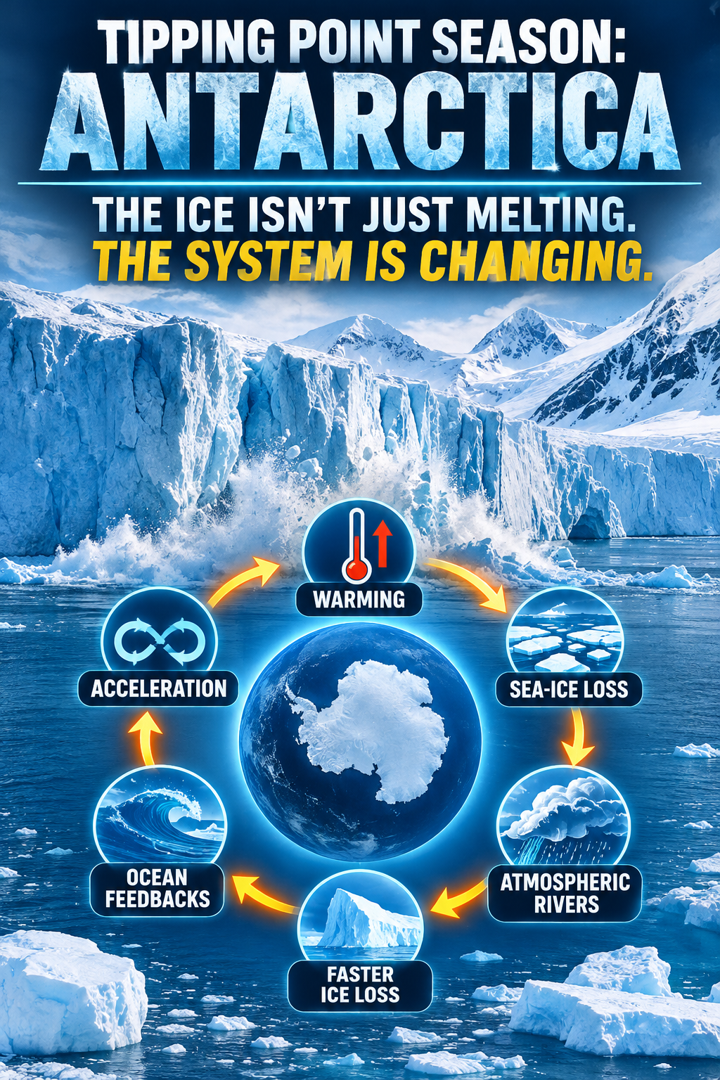
🌎 TIPPING POINT SEASON: ANTARCTICA
THE ICE ISN’T JUST MELTING. THE SYSTEM IS CHANGING.
Antarctica is sending some unmistakable warning signals.
Record-low sea-ice coverage. Rapid glacier retreat. Deteriorating ice shelves. Changing ocean circulation. Increasingly important atmospheric rivers. And new research identifying mechanisms that can accelerate ice-sheet instability.
But the biggest concern isn’t any single event. It’s how these processes interact.
🔥 Warming oceans weaken ice shelves. 🧊 Sea-ice loss increases solar energy absorption. 🌧️ Atmospheric rivers transport heat and moisture toward Antarctica. 🌊 Changing ocean conditions influence glacier stability and ice discharge. ⚠️ Coupled feedbacks can amplify the changes.
Our Nonlinear Climate Acceleration Hypothesis examines how these processes interact:
Antarctica also demonstrates why looking at individual climate indicators can be misleading. Increased snowfall can temporarily offset ice loss while glaciers continue discharging ice into the ocean.
The question isn’t simply how much ice Antarctica is losing.
It’s how quickly the interconnected systems governing its ice, atmosphere, and ocean are changing.
This is another installment in our Tipping Point Season Hunting Manual, exploring the evidence behind climate tipping points, feedback coupling, and the emerging planetary Domino Effect.
One planet. One interconnected climate system. Multiple tipping points.
The ice isn’t just melting. The system is changing.
Antarctica is experiencing a profound change in its climate and ice dynamics. Record-low sea-ice coverage, rapidly retreating glaciers, weakening ice shelves, and changing atmospheric circulation are revealing a complex system under increasing stress.
Several developments make Antarctica particularly important to our investigation of climate tipping points:
The eastern ice shelf of Thwaites Glacier is losing its structural integrity, threatening its ability to restrain the grounded ice behind it.
Hektoria Glacier experienced approximately 25 kilometers (15 miles) of retreat in just 15 months, including the fastest observed retreat of grounded glacier ice in the modern satellite record.
Antarctic sea ice reached its third-lowest winter maximum in the satellite record in September 2026.
Atmospheric rivers are increasingly important to Antarctic precipitation and ice-sheet mass balance.
New research identifies rate-induced tipping as a mechanism through which rapidly changing climate conditions can destabilize marine-based ice sectors before traditional equilibrium thresholds are reached.
At the same time, new research provides an important qualification: some exposed ice cliffs stabilize after rapidly retreating, demonstrating that not every destabilization produces an unstoppable collapse.
The larger concern is the interaction of multiple processes: warming oceans, atmospheric heating, changing wind patterns, sea-ice retreat, precipitation, and glacier dynamics.
Antarctica is not simply losing ice. Its interconnected systems are changing.
1. Thwaites Glacier: The Weakening Buttress
Thwaites Glacier remains one of the most consequential components of the global sea-level system.
Often called the “Doomsday Glacier,” Thwaites is particularly vulnerable because its grounded ice rests on a bed that deepens inland. This geometry makes retreating grounding lines susceptible to marine ice-sheet instability.
Its floating eastern ice shelf provides an important restraining force, slowing the movement of grounded ice toward the ocean.
But that structural support is deteriorating.
Ice Shelf Disintegration
The eastern ice shelf is experiencing extensive fracturing and structural deterioration. Its connection to an underwater ridge has been weakening, reducing its ability to restrain the glacier.
As the ice shelf loses structural integrity, the grounded glacier becomes increasingly exposed to accelerated discharge into the ocean.
Loss of Buttressing
The floating ice shelf acts like a cork restraining the movement of the glacier behind it.
When that support weakens, the grounded ice can accelerate toward the ocean. This is particularly dangerous where the grounding line retreats into deeper water.
Grounding-Zone Melting
Warm ocean water reaches beneath floating ice and attacks the glacier near its grounding zone.
Tidal pumping and changing ocean circulation can transport relatively warm water farther beneath the ice, increasing basal melting and weakening the connection between grounded and floating ice.
The important issue is not simply how much ice melts at the surface.
It is the loss of structural support that allows enormous quantities of grounded ice to move into the ocean.
Thwaites demonstrates how ocean warming, ice-shelf deterioration, grounding-line retreat, and glacier acceleration can interact as reinforcing processes.
2. Record-Breaking Glacier Retreat and Iceberg Movement
Antarctica is experiencing changes that challenge assumptions about the speed of glacier retreat.
Hektoria Glacier: 15 Miles in 15 Months
Between January 2022 and March 2023, Hektoria Glacier retreated approximately 25 kilometers (15 miles).
During one two-month period, its grounded terminus retreated more than 8 kilometers (5 miles).
NASA identified this as the highest rate of grounded glacier-ice loss observed in the modern record.
This is particularly important because the retreat was not simply the disappearance of floating ice. It involved the rapid withdrawal of grounded glacier ice, which directly contributes to sea-level rise.
The Hektoria event demonstrates how quickly glacier dynamics can change when floating ice support is lost.
The enormous iceberg A-81, approximately 600 square miles in area, broke away from Antarctica’s Brunt Ice Shelf in January 2023. After spending more than three years moving through the Weddell Sea, it traveled north toward South Georgia.
By October 2026, NASA satellite observations showed the iceberg approaching South Georgia, approximately 1,400 miles from its point of origin.
This journey illustrates the enormous scale of Antarctic ice movement and the influence of ocean circulation on the redistribution of ice throughout the Southern Ocean.
Rate-Induced Tipping: A New Dimension of Ice-Sheet Instability
An October 20, 2026 study published in Nature Geoscience identifies an important mechanism known as rate-induced tipping. Traditional tipping-point analysis often focuses on whether a system crosses a particular critical temperature or equilibrium threshold.
Rate-induced tipping introduces another possibility: the climate system can change so rapidly that stabilizing processes cannot respond quickly enough. In Antarctic ice sheets, the relevant stabilizing mechanism includes the gradual uplift of the underlying bedrock as ice is removed.
If warming and ice loss outpace that adjustment, grounding lines can retreat into vulnerable terrain and initiate self-sustaining retreat before the traditional equilibrium threshold is reached.
The study identifies particular vulnerability in the Recovery and Aurora subglacial basins of East Antarctica.
The rate at which the climate changes can be just as important as the eventual temperature reached.
3. Antarctic Sea Ice: A Major Change in the Energy Balance
On September 14, 2026, Antarctic sea ice reached its annual winter maximum at approximately 17.59 million square kilometers. This was the third-lowest winter maximum in the satellite record.
The significance extends beyond the amount of missing ice.
Between 1979 and 2014, Antarctic sea ice exhibited a modest overall increase, although considerable regional and year-to-year variability existed. That pattern reversed beginning in 2015–2016.
Since then, Antarctic sea ice has experienced repeated periods of unusually low coverage, including record-low seasonal minimums and maximums.
The 2026 observations reinforce the significance of this shift. Antarctic climate feedbacks are increasingly self-reinforcing, while the system’s remaining resilience appears insufficient to reverse the deterioration. These developments signal an increasing risk of approaching critical tipping points.
The Albedo Feedback
Sea ice reflects incoming solar radiation. Dark ocean water absorbs considerably more energy.
As sea ice retreats:
More dark ocean becomes exposed.
More incoming solar radiation is absorbed.
Ocean-atmosphere heat and moisture exchange changes.
Atmospheric moisture availability increases in affected regions.
Regional temperatures and precipitation patterns respond.
This creates opportunities for reinforcing feedbacks between ocean warming, sea-ice loss, atmospheric moisture, and ice-sheet behavior.
The Southern Ocean is not simply surrounding Antarctica. It is an integral part of the global energy-distribution system.
4. The October 2026 Temperature Record: Atmospheric Rivers and Foehn Winds
On October 2026, Ukrainian researchers at the Akademik Vernadsky Antarctic research station recorded an air temperature of +11.1°C (52°F).
This established a new October temperature record for the station’s vicinity, surpassing the previous October record of +7.9°C set in 1968. Even more remarkable was the speed of the temperature change.
The air warmed from +1.2°C to +11.1°C in approximately two and a half hours.
At the same time:
Wind speed increased from 1.5 to 13.1 meters per second.
Relative humidity dropped from 90% to 54%.
Wind direction changed.
These observations are consistent with an intense foehn wind event.
Foehn Winds: Rapid Atmospheric Heating
Foehn winds develop when air crosses a mountain range, loses moisture as it rises, and descends on the opposite side. As the descending air is compressed by increasing atmospheric pressure, its temperature rises. The result can be an exceptionally rapid increase in local temperature.
In Antarctica, these winds can accelerate surface melting and alter the stability of snow and ice.
Atmospheric Rivers: Transporting Heat and Moisture
The Ukrainian National Antarctic Scientific Center identified an atmospheric river as a possible contributing factor to the October event. Atmospheric rivers are concentrated corridors of atmospheric moisture that transport enormous quantities of water vapor across long distances. They are important because they connect distant oceanic and atmospheric conditions with precipitation and temperature changes in polar regions.
The event illustrates the kind of atmospheric interaction known as coupled feedbacks and the domino effect.
5. Atmospheric Rivers: The Antarctic Ice-Mass Paradox
One of the most important developments in Antarctic climate research appeared in February 2026 in Communications Earth & Environment.
The study, “Atmospheric rivers and winter sea ice drive recent reversal in Antarctic ice mass loss,” examined an unexpected development. Despite continued increases in dynamically driven ice discharge from outlet glaciers, satellite measurements showed a substantial slowdown in overall Antarctic ice-mass loss and a period of net mass gain beginning around 2020.
The explanation was increased snowfall.
Atmospheric rivers, strengthened westerly winds, and changing atmospheric circulation increased precipitation over large areas of Antarctica. That additional snowfall temporarily offset ice losses occurring through glacier discharge.
The Paradox
Antarctica can gain overall ice mass while individual glaciers continue losing ice at accelerating rates.
The study found that:
Atmospheric rivers became more frequent and intense after 2020.
Increased precipitation produced substantial positive surface-mass-balance anomalies.
Glacier discharge continued to accelerate.
Increased snowfall temporarily exceeded the additional losses from ice discharge.
Reduced sea ice contributed to increased precipitation, but large-scale atmospheric circulation was the dominant driver.
The researchers estimated that sea-ice reduction accounted for approximately 11% of the recent winter surface-mass-balance increase.This is an excellent example of why examining only one climate indicator can produce an incorrect conclusion.
A temporary increase in Antarctic ice mass does not establish that the ice sheet has recovered or that its underlying structural instability has disappeared.
The same atmospheric process can contribute to both temporary ice accumulation and longer-term ice destabilization.
Atmospheric rivers transport moisture that becomes snowfall, but warm and moist atmospheric intrusions can also contribute to surface melting and changes in ice dynamics.
6. Ice Cliff Resilience: An Important Scientific Qualification
A major four-year satellite investigation published in Science on October 15, 2026 examined more than 15,000 Antarctic ice cliffs.
Researchers from MIT and Woods Hole Oceanographic Institution investigated whether exposed ice cliffs necessarily initiate runaway collapse after floating ice shelves disappear.
Traditional marine ice-cliff instability models suggested that cliffs exceeding approximately 100 meters could collapse under their own weight, exposing taller inland cliffs and triggering a self-sustaining retreat.
The observations revealed a more complicated process.
Researchers found that:
Taller cliffs can retreat faster than previously modeled.
Their collapse does not necessarily trigger an unstoppable chain reaction.
Dynamic thinning and retreat into regions with lower ice-thickness gradients can stabilize retreat.
Cliff stability depends on more than height alone.
This is an important qualification to worst-case ice-sheet projections. It does not eliminate the danger of Antarctic ice loss. In fact, the researchers found that some cliffs retreat faster than earlier models predicted, potentially increasing short-term ice loss and sea-level contributions.
The finding demonstrates that climate feedbacks are not necessarily unlimited. Some processes provide stabilizing responses even while other components of the system continue deteriorating.
The important distinction is between temporary stabilization and recovery of the larger ice system.
7. How Antarctica Fits the Nonlinear Climate Acceleration Hypothesis
The most important implication is that Antarctic climate change cannot be adequately understood by examining temperature or ice loss independently.
Our research framework identifies three stages of climate change:
First Derivative: Climate Change
The planet is warming.
Second Derivative: Climate Acceleration
The rate of climate change is increasing.
Third Derivative: Climate Jerk
The rate of acceleration itself is changing.
Climate Jerk is particularly relevant when examining abrupt changes in atmospheric circulation, precipitation, wind patterns, glacier dynamics, and ice-sheet stability. A rapidly changing climate system does not necessarily produce a smooth increase in temperature.It can produce abrupt transitions in the behavior of interconnected systems.
The broader feedback-coupling model describes the progression:
Antarctica provides important examples of these processes:
Our framework
Antarctic manifestation
Warming
Record October station temperature and ocean warming
Feedback activation
Sea-ice retreat and changing ocean-atmosphere energy exchange
Coupling
Atmospheric rivers, foehn winds, moisture, and ice dynamics
Amplification
Surface melting, basal melting, and glacier discharge
Threshold
Ice-shelf structural deterioration and grounding-line instability
Cascade
Glacier retreat, sea-level rise, freshwater redistribution, and further Earth-system disruption
The important question is not simply whether each individual process is accelerating.
It is whether their interactions are increasing the rate and magnitude of change throughout the larger system.
8. The Antarctic Domino Effect: Connecting the Planetary System
Antarctica is connected to the rest of the planet through ocean circulation, atmospheric circulation, and the global energy balance.
Changes in one region can influence conditions thousands of miles away.
Consider the following interconnected processes:
OCEAN WARMING ↓ CHANGES IN ATMOSPHERIC CIRCULATION ↓ ATMOSPHERIC RIVER FREQUENCY AND INTENSITY ↓ ANTARCTIC HEAT AND MOISTURE TRANSPORT ↓ SEA-ICE AND ICE-SHEET CHANGES ↓ ALBEDO, FRESHWATER, AND OCEAN-CIRCULATION FEEDBACKS ↓ FURTHER EARTH-SYSTEM DISRUPTION
These are not necessarily one-way processes. Many operate simultaneously and influence one another. A particularly important new development appeared in Nature Climate Change on October 28, 2026. Researchers documented a reversal in the long-term trends of Antarctic Intermediate Water, a water mass that plays an important role in global ocean circulation.
They linked the change to the dramatic decline in Antarctic sea ice since 2016.
The study identified changes in freshwater input, ocean stratification, salinity, and water-mass properties, demonstrating that Antarctic sea-ice changes are affecting ocean processes extending well beyond the immediate polar region.
This is another important example of the planetary connections central to the Domino Effect research.
This relationship examines how accumulated ocean energy translates into structural ice loss and accelerated glacier movement.
3. Albedo × Ocean Heat × Atmospheric Moisture
This relationship examines how disappearing reflective surfaces influence energy absorption, ocean-atmosphere exchange, and atmospheric moisture transport.
Conclusion: We Are Not Simply Watching the Ice Melt
Antarctica provides one of the clearest opportunities to examine how multiple climate-sensitive systems interact.
The evidence is not limited to rising temperatures.
We are observing:
Rapid glacier retreat.
Deteriorating ice-shelf structures.
Repeatedly low Antarctic sea-ice coverage.
Increasingly important atmospheric-river activity.
Changes in ocean circulation and water-mass properties.
Rate-dependent ice-sheet instability.
Temporary stabilization mechanisms that can mask continuing ice loss.
The October 2026 temperature record provides another illustration of how rapidly atmospheric conditions can change in the Antarctic environment. But the larger story is the interaction between these processes.
Atmospheric rivers can increase snowfall while transporting heat and moisture. Sea-ice loss changes the energy balance and ocean-atmosphere exchange. Ocean warming attacks ice shelves from below. Glacier retreat changes the distribution of ice and freshwater. Changes in ocean properties can influence circulation throughout the planet.
These processes do not operate independently.
They are interconnected components of one planetary climate system.
Our central proposition is that climate acceleration must be understood through the interaction of these processes—not simply by measuring the temperature of the atmosphere. The greatest danger may not be one isolated tipping point. It may be the interaction of multiple tipping elements, each changing the conditions under which the others operate.
This is what we are hunting for during Tipping Point Season. We are not simply watching the ice melt. We are watching for evidence that the climate system is beginning to behave differently.
One planet. One interconnected climate system. And an increasingly important question:
How quickly are the connections between climate tipping points changing the trajectory of the entire Earth system?
Tipping Point Season Hunting Manual — Antarctic Case Study
Climate Change Is Accelerating: From Acceleration to Climate Jerk and System-Wide Feedback Coupling
By Daniel Brouse and Sidd Mukherjee
Overview
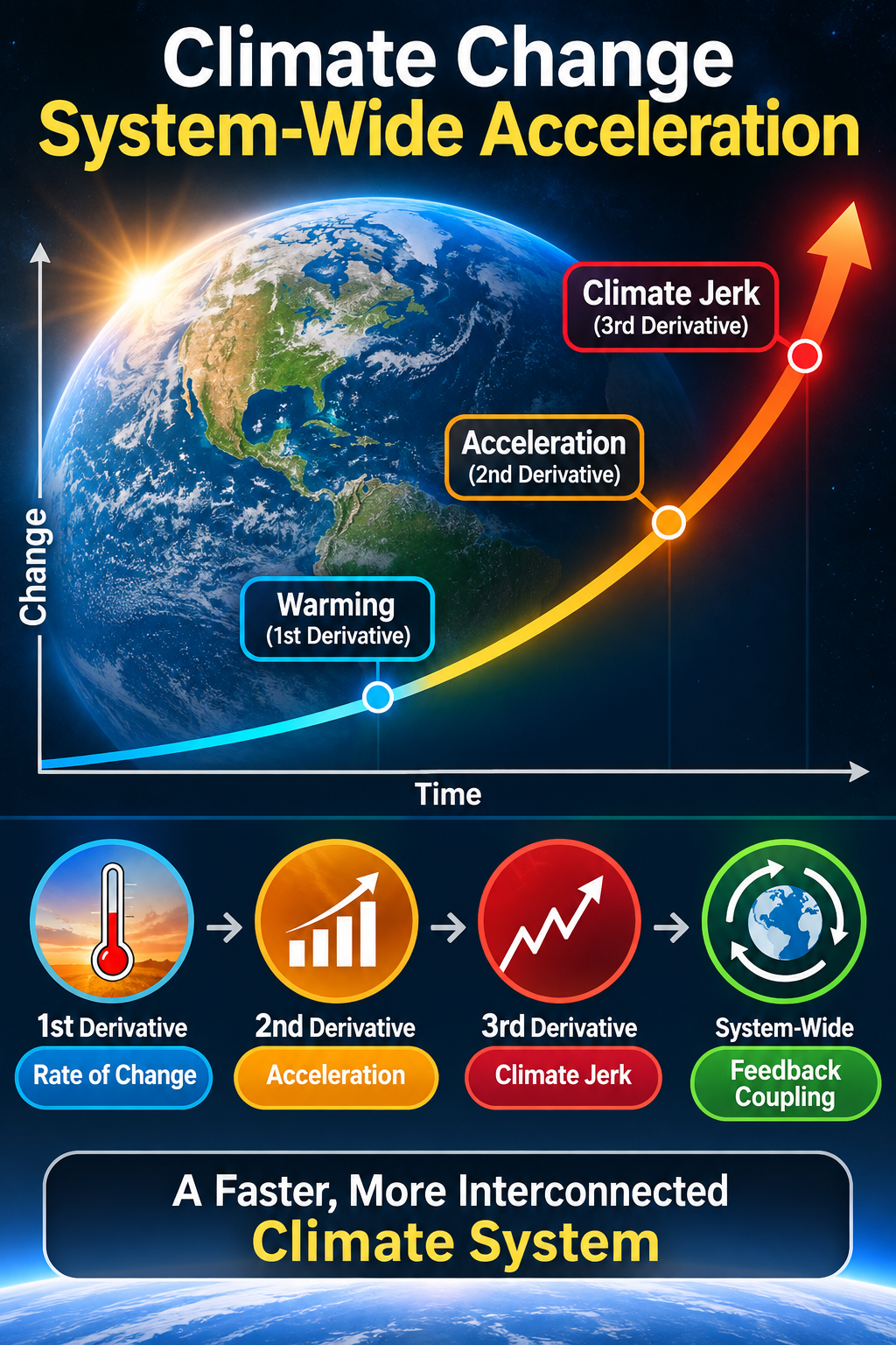
🌎 CLIMATE CHANGE SYSTEM-WIDE ACCELERATION
How fast is climate change changing?
Climate change isn’t simply accelerating. The acceleration itself is increasing.
In the paper, “Climate Change Is Accelerating: From Acceleration to Climate Jerk and System-Wide Feedback Coupling,” Daniel Brouse and Sidd Mukherjee examine the progression from ordinary warming to nonlinear acceleration, third-derivative behavior (Climate Jerk), and increasingly interconnected climate feedbacks.
Our research examines several critical developments:
📈 1st Derivative: The rate of climate change.
📈 2nd Derivative: Acceleration — the rate of change is increasing.
🚨 3rd Derivative: Climate Jerk — acceleration is increasing.
🌎 System-Wide Coupling: Multiple climate feedbacks interact and amplify changes throughout the Earth system.
Our 2022–2026 analysis identifies a particularly important Albedo–Cloud–Ocean Heat Content feedback triad, accounting for 39.6% of the calculated climate jerk surge weight.
The implications are significant: examining individual climate indicators is no longer enough. We must increasingly measure how the entire climate system is changing, how its feedbacks are interacting, and how rapidly those interactions are evolving.
We are moving from measuring climate change to measuring the changing dynamics of climate change itself.
The question is no longer just how much the planet is warming.
It’s how fast the processes driving that warming are changing.
The rate at which Earth’s climate is changing is becoming increasingly apparent. More importantly, the rate at which climate change itself is accelerating is becoming easier to observe and measure.
For much of the twentieth century, detecting this acceleration was difficult. Individual climate indicators changed relatively slowly, and the climate system was generally analyzed as a collection of separate variables rather than as an interconnected, dynamically evolving system. Conventional climate projections frequently emphasized approximately linear trends, even as the underlying physics allowed for nonlinear behavior.
By the 1990s, the scientific understanding of climate change was beginning to evolve. Michael E. Mann, Raymond S. Bradley, and Malcolm K. Hughes published their influential hockey-stick reconstruction of historical temperatures, demonstrating the unusual magnitude of modern warming. Meanwhile, the scientific understanding of radiative forcing, developed through more than a century of research, was becoming formalized as a central climate metric in the IPCC’s 1990 First Assessment Report.
The emerging challenge was no longer simply determining whether Earth’s climate was warming. It was determining whether the warming process itself was accelerating.
By the late 1990s, changes in individual climate indicators were becoming increasingly apparent. Scientists such as James Hansen were documenting evidence of accelerating global warming, while researchers, including Sidd Mukherjee and Daniel Brouse, were investigating nonlinear behavior in sea-level rise.
Sea-level rise provided an especially useful example because it demonstrated how a relatively gradual physical process could increase its rate of change over time.
Approximate historical global mean sea-level rates illustrate this progression:
Period
Approximate annual rise
Pre-1900
0.75 mm/year
1900–2000
1.5 mm/year
These approximate historical values illustrate a doubling of the annual rate over roughly a century. Subsequent observations have documented further acceleration.
This is known as second-derivative behavior, or acceleration.
In mathematical terms:
First derivative (rate of change):
dI/dt
Second derivative (acceleration):
d²I/dt²
Where:
I represents a climate indicator.
The first derivative measures its rate of change.
The second derivative measures the rate at which that rate changes.
When the second derivative is positive, the indicator is accelerating.
Climate change was no longer simply progressing. Its rate of change was increasing, demonstrating nonlinear behavior consistent with exponential growth in certain climate processes.
2. Third-Derivative Behavior: Climate Jerk
By the 2020s, an additional and more consequential pattern was becoming observable: the acceleration of individual climate indicators was itself increasing.
This is known as third-derivative behavior, or jerk.
The mathematical expression for climate jerk is:
J(t) = d³I/dt³
Where:
J(t) represents climate jerk at time t.
I represents a climate indicator.
t represents time.
The first derivative measures the rate of change.
The second derivative measures acceleration.
The third derivative measures the change in acceleration.
A positive third derivative indicates that acceleration is increasing.
Multiple climate indicators have exhibited increasingly pronounced nonlinear behavior, including:
Flooding and extreme precipitation
Atmospheric moisture content
Ocean heat content
Rossby wave amplification
Sea-level rise
Nighttime temperatures and extreme heat
Ice-sheet mass loss
Glacial retreat
Permafrost thaw
Wildfire activity
Wet-bulb temperature extremes
These indicators are not independent. They interact through physical processes that redistribute energy, moisture, and heat throughout the Earth system.
Consequently, acceleration in one component can influence the behavior of others, creating interconnected feedback pathways.
The significance of climate jerk is that it provides a mathematical framework for describing a system in which the rate of acceleration is itself increasing.
3. Whole-System Magnitude: From Individual Indicators to Coupled Feedbacks
In 2026, our research, Climate Jerk Surge: Albedo–Cloud–Ocean Heat Content Feedback Triad, examined an important development in climate-system behavior.
The analysis demonstrated that recent changes in climate dynamics are being expressed not simply through continued warming, but through increasing synchronization among multiple radiative and thermal feedback pathways.
A 2022–2026 analysis identified a pronounced increase in calculated coupling jerk across a six-variable climate system.
The strongest contributions were concentrated in a closely interconnected Albedo–Cloud–Ocean Heat Content feedback triad.
The three-way feedback relationship accounted for 39.6% of the displayed surge weight.
This highlights the importance of interactions among Earth’s reflectivity, cloud behavior, and accumulated ocean heat.
This represents a shift in the analytical approach: rather than examining climate indicators exclusively as separate measurements, we are examining how their interactions contribute to the behavior of the entire climate system.
The analysis also highlights the importance of emerging or previously underappreciated feedback pathways, including declining low-level cloud cover and ozone-related atmospheric and ecological forcing.
These processes are particularly important because they can influence the Earth’s energy balance, vegetation productivity, carbon uptake, and the strength of existing feedback mechanisms.
Their increasingly apparent behavior over the relatively short 2022–2026 observation window makes them important subjects for continued investigation.
4. The Transition to Whole-System Measurement
One of the most important developments in climate analysis is the transition from measuring changes in individual indicators to measuring changes in the behavior of the interconnected climate system.
As individual indicators become increasingly nonlinear, distinguishing their underlying acceleration from natural variability, measurement uncertainty, and interacting processes becomes more difficult.
At the same time, the cumulative effects of these processes become increasingly apparent in whole-system measurements.
Earth’s energy imbalance is particularly important.
More than 90% of the excess energy accumulating in the climate system is entering the oceans. Ocean heat content therefore provides a powerful measure of the cumulative consequences of the Earth’s energy imbalance.
The advantage of whole-system analysis is that it captures the combined effects of multiple interacting processes rather than relying exclusively on the behavior of individual indicators.
This is especially important when feedbacks become coupled and changes in one component amplify changes in another.
The result is a climate system whose behavior cannot be adequately described by examining individual trends in isolation.
5. The Bigger Picture: Measuring How Quickly Climate Change Is Changing
The progression from first-derivative warming to second-derivative acceleration and third-derivative jerk represents an increasingly sophisticated understanding of climate-system behavior.
First derivative — Rate of change
dI/dt
The climate is warming, and individual indicators are changing.
Multiple climate processes increasingly interact, synchronize, and amplify changes throughout the Earth system.
The central issue is no longer simply how much Earth’s temperature has increased, or even how quickly it is increasing.
It is how quickly the processes driving climate change are themselves changing.
This distinction matters because a climate system experiencing increasing acceleration and increasingly interconnected feedbacks behaves differently from one following a relatively stable, linear trajectory.
We are moving from measuring climate change to measuring the changing dynamics of climate change itself.
That is the significance of climate jerk and whole-system feedback coupling.
Advances in technology, modeling, and artificial intelligence have significantly improved our ability to understand and track the accelerating dynamics of climate change. These tools have provided new insight into how quickly complex systems can evolve—and how difficult it may be to keep pace with that acceleration.
Our analysis suggests that the climate–economic system is now exhibiting third-derivative behavior, indicating that not only are impacts increasing, and accelerating, but the acceleration itself is increasing. This places the system within a singularity-like regime, characterized by nonlinear amplification, rising instability, and reduced predictability.
Historically, such transitions were assumed to unfold over tens of thousands to millions of years based on paleoclimate evidence. However, current observations indicate that these dynamics may be occurring on dramatically compressed timescales, raising the possibility that singularity-like behavior could emerge within contemporary time horizons.
Given the importance and accessibility of these findings, this work is presented in three formats:
Each version conveys the same core insight: complex, coupled systems can shift rapidly from stable to unstable behavior, and understanding this transition is critical to anticipating future climate and economic risk.
Singularity in Climate Dynamics: The Ultimate Acceleration of Change
Why the Age of Artificial Intelligence Requires a New Economic Model
By Daniel Brouse
The Economic Challenge of Artificial Intelligence
We need a new economic model that separates people’s ability to earn a living from the necessity of working for a living.
As artificial intelligence (AI) and automation transform the economy, traditional employment may no longer provide a reliable source of income for everyone. Machines can increasingly perform tasks that once required human labor, raising productivity while potentially eliminating jobs and weakening the link between employment and economic security.
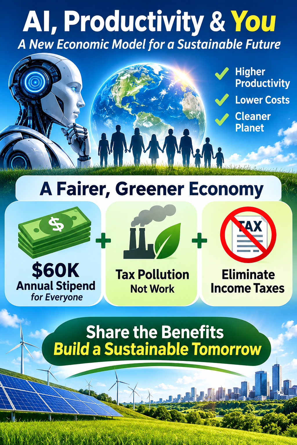
One approach worth serious consideration is a $60,000 annual government stipend per person, funded in part by taxing pollution while eliminating income taxes. This would shift the tax burden away from human productivity and toward activities that impose environmental costs, while providing people with a more secure share of the economy’s productive output.
This is a proposed economic model, not an established policy. Its implementation would require careful consideration of funding, inflation, eligibility, existing public benefits, and the distribution of economic gains.
The Productivity and Disinflation Wildcard
Another important variable is the relationship between productivity gains and disinflation.
AI-driven improvements in productivity and efficiency could sharply reduce the cost of producing goods and services. As automation reduces labor requirements and technological advances improve resource utilization, prices could decline even as total economic output increases.
This creates an important possibility: We could produce more while requiring less human labor and fewer resources.
If these productivity gains translate into lower consumer prices, a given income could purchase more goods and services. The result could be a substantial improvement in living standards, provided the benefits reach consumers rather than being captured primarily as corporate profits.
However, lower production costs do not automatically translate into lower prices. Market competition, ownership, energy costs, access to resources, and corporate pricing decisions will influence how much of the savings consumers receive. Nor does greater productivity guarantee that every sector will experience falling prices.
The central economic challenge is to ensure that the benefits of technological progress are broadly shared rather than concentrated among a small number of business owners and investors.
We cannot stop technological progress, but we can redesign our economic system to distribute its benefits more equitably.
Global Responses: Policies Already Under Consideration
The economic transition driven by AI is not a distant possibility. It is already underway. Governments worldwide are considering different ways to address technological disruption, economic inequality, and the distribution of productivity gains.
These initiatives differ in their objectives and scope. Some involve direct cash payments, others explore basic income, and still others seek to capture more public revenue from digital economic activity. They provide examples of the policy options emerging as governments respond to a changing economy.
Taiwan: Proposed Cash Distribution
In August 2026, President Lai Ching-te announced plans for a NT$10,000 cash payment to eligible residents through the 2027 budget. The government cited strong economic growth driven by global demand for AI-related products and sought to share some of the benefits of that growth.
The proposal was referred for legislative review in October 2026. The planned distribution should therefore be understood as a proposed measure, not a completed payment program.
European Union: Debate Over AI Taxation
European policymakers and tax experts are examining how AI-driven automation could erode payroll-tax revenue used to fund pensions, healthcare, and other social programs.
Proposals include shifting more taxation toward corporate profits and exploring ways to capture economic value generated by AI. Direct taxation of AI systems or AI-generated work has also entered the policy debate, although no EU-wide AI-worker tax has been enacted.
The underlying concern is straightforward: If machines perform a growing share of economically valuable work, governments may need to reconsider how they fund public services traditionally financed through taxes on human employment.
South Korea: Basic-Income Proposals
South Korean political leaders, including Lee Jae-myung, have advocated basic-income policies amid concerns about economic inequality, automation, and employment disruption.
These proposals reflect a broader debate about whether traditional employment-based income distribution will remain adequate as AI changes the relationship between labor, productivity, and economic output.
The policy question is how to ensure that technological progress improves living standards across society, including for people whose jobs are displaced or whose bargaining power declines.
The Marshall Islands: Nationwide Universal Basic Income
In November 2025, the Marshall Islands launched its ENRA universal basic income program, providing regular distributions to eligible citizens.
The program uses multiple payment channels, including a dedicated digital wallet. It demonstrates how modern financial infrastructure can support nationwide cash transfers.
The program is funded through the country’s Compact Trust Fund rather than an AI-specific tax. Although it was not created as a response to AI-driven unemployment, it provides a real-world example of a government implementing regular, broadly distributed public payments.
Kenya: Taxation of the Digital Economy
Kenya has pursued taxation of digital economic activity as governments seek to capture revenue from an increasingly digital global economy.
In December 2024, Kenya replaced its 1.5% digital services tax with a 3% significant economic presence tax applying to qualifying nonresident digital businesses, subject to the relevant rules.
This approach illustrates one way to tax economic activity that may not fit traditional models of physical presence and employment. It is not specifically an AI tax or a universal basic-income funding mechanism, but it contributes to the broader discussion about how tax systems must evolve as technology changes how businesses generate revenue.
The United States: A Proposed AI Sovereign Wealth Fund
In June 2026, Senator Bernie Sanders introduced the American AI Sovereign Wealth Fund Act, proposing public ownership of a portion of qualifying AI companies through a federally managed sovereign wealth fund.
The proposal calls for a one-time transfer of 50% of the stock of qualifying AI companies with at least $200 million in annual AI sales. The fund would hold these shares and distribute public benefits, including annual dividends, while supporting priorities such as healthcare, education, and housing.
The legislation remains a proposal, not enacted law. Its approach differs from a universal stipend funded through environmental taxation, but it addresses the same fundamental question: Who should benefit from the wealth created by increasingly powerful technologies?
A sovereign wealth fund could give the public a direct financial stake in AI-generated economic value. A universal stipend funded through taxation would pursue a similar distributional objective through a different mechanism.
Both approaches raise important questions about implementation, governance, funding, and the long-term relationship between private ownership and public benefit.
The Broader Economic Implication
These examples represent different approaches to a common challenge: distributing the benefits of economic growth when technological progress reduces the need for human labor.
They are not all AI-specific initiatives, and none establishes that a permanent $60,000 annual stipend is already a widely adopted policy. Nevertheless, they demonstrate that governments are exploring alternatives to relying exclusively on employment-based income and conventional payroll taxation.
The essential question is becoming increasingly important:
As AI and automation increase productivity while reducing the need for human labor in some occupations, how should society distribute the resulting economic gains and finance essential public services?
Universal basic income, public dividends, sovereign wealth funds, digital-economy taxation, and environmental tax reform are among the approaches worth examining.
Productivity, Human Welfare, and Environmental Sustainability
AI presents both an economic challenge and an opportunity.
If technological progress allows society to produce more goods and services with fewer labor hours and less resource consumption, the potential benefits extend beyond corporate profitability. People could enjoy greater economic security, more free time, lower living costs, and improved access to essential goods and services.
Realizing those benefits requires more than technological innovation. It requires economic institutions that translate productivity gains into broadly shared prosperity.
Environmental taxation offers a complementary opportunity. Taxing pollution while reducing or eliminating taxes on income could encourage cleaner production while reducing the financial penalty on human work. The actual environmental and economic results would depend on tax design, implementation, and how revenues are distributed.
The goal should be an economic system that rewards innovation, supports human welfare, and accounts for environmental costs rather than treating them as someone else’s problem.
Conclusion: Adapt the Economy to the Technology
The transition to AI-driven productivity is already underway. Attempting to preserve every existing job or slow technological obsolescence indefinitely is not a sustainable strategy.
The more important task is to prepare society for an economy in which human labor may no longer be the primary constraint on production.
A guaranteed annual stipend, pollution-based taxation, reduced reliance on income taxes, and mechanisms for distributing AI-generated wealth are possible elements of a new economic model. Productivity-driven disinflation could further improve affordability if lower production costs translate into lower consumer prices.
None of these outcomes is automatic. They depend on policy choices, economic incentives, market structures, and how society chooses to distribute the benefits of innovation.
We cannot stop technological progress. We can decide whether its benefits are concentrated among a few or shared throughout society.
The objective should be clear: an economy that turns technological productivity into human prosperity while advancing environmental sustainability.
Note From the Author
We are likely facing the most profound economic revolution in human history, and we are dangerously unprepared for its consequences.
Ironically, the U.S. has ignored our most significant existential risk: climate change. The acceleration of Earth’s energy imbalance is already well underway, with consequences that extend far beyond rising temperatures. The economic damage is enormous and growing, with estimates reaching trillions of dollars annually and potentially tens of trillions by midcentury, depending on the scenario and methodology.
Here’s the irony: AI may be our best hope for solving the climate crisis. Its ability to accelerate scientific research, optimize energy systems, improve efficiency, and develop new technologies could help us respond at the scale and speed required.
But just as with climate change, technological capability alone isn’t enough. We need the political will and economic framework to put those capabilities to work for the public good.
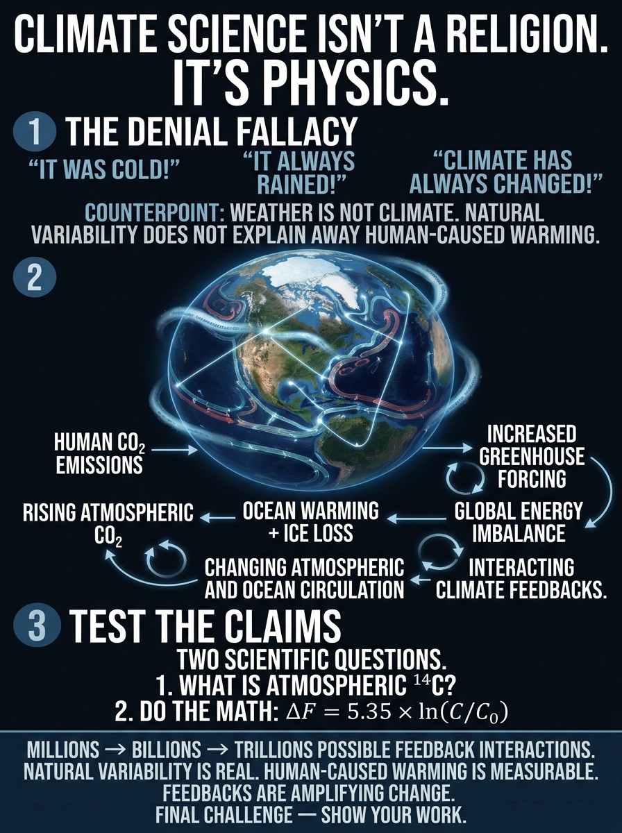
Weather too hot? Weather too cold? Too much rain? Drought?
Climate deniers love to ridicule the science while ignoring the physics. But climate science isn’t about blaming every weather event on global warming. It’s about understanding the measurable physical processes connecting Earth’s atmosphere, oceans, ice, and ecosystems.
📊 10 FRAMES. FOLLOW THE PHYSICS. TEST THE CLAIMS.
This slideshow breaks down the science:
🌍 Human CO₂ emissions and rising atmospheric concentrations.
🔥 Greenhouse forcing and Earth’s growing energy imbalance.
🌊 Ocean warming, melting ice, and changing circulation.
🌀 Interconnected climate feedbacks that can amplify change.
🔬 Atmospheric carbon-14 and the physics of CO₂ radiative forcing.
🦋 The butterfly effect: how changes in interconnected systems can propagate far beyond their origin.
Natural variability is real. Climate has changed throughout Earth’s history. Neither fact explains away the measurable human contribution to today’s global warming.
The challenge to climate deniers is simple: If you dispute the science, engage with the evidence. Explain the physical mechanisms. Quantify your alternative explanation. Show your work.
Laughing emojis aren’t scientific evidence. Neither are unsupported claims about research funding.
CLAIMS AREN’T EVIDENCE. FOLLOW THE DATA.
MILLIONS → BILLIONS → TRILLIONS OF POSSIBLE FEEDBACK INTERACTIONS.
Feedback coupling is emerging. Understanding how these connections develop, interact, and amplify change is one of the major challenges in climate science.
Science Denier Response of the Day (Feel free to reuse and share.)
Let’s have a pop quiz to test your scientific literacy—and whether your laughing emojis can substitute for scientific evidence.
1. Explain atmospheric ¹⁴C concentrations. What do they reveal about the sources of rising atmospheric CO₂?
2. Apply your answer using the CO₂ radiative forcing formula:
ΔF = 5.35 × ln(C/C₀) [W/m²]
Explain what this equation tells us about the radiative forcing caused by rising atmospheric CO₂ concentrations.
If natural variability is your preferred explanation, demonstrate it with evidence and quantitative analysis. Assertions, conspiracy theories about research funding, and laughing emojis are not scientific arguments.
*Show your work.* (If you are totally ignorant, reply with your foolish emojis.)
—————————————————–
Full Conversation
Climate denier said:
“Weather too hot? Global warming. Weather too cold? Global warming. Too much rain? Global warming. Drought? Global warming. What’s the question? Doesn’t matter. The answer’s the same. Global warming. To true believers in the global warming religion, everything is a sign.” IBD
I replied:
What? You need to stop following your pseudoscience gods and listen to scientists. This is what we actually say: Polar amplification → weakened equator-to-pole temperature gradients → reduced thermal contrast that helps drive and stabilize large-scale atmospheric circulation → accelerated Greenland and Arctic ice melt → freshwater input into the North Atlantic and reduced salinity/density of surface waters → disruption and potential weakening of the Atlantic Meridional Overturning Circulation (AMOC) → reorganization of North Atlantic pressure fields and storm tracks → greater jet-stream waviness, slower progression, and amplified Rossby-wave behavior → more persistent blocking patterns, omega blocks, and meridional flow → stalled atmospheric rivers, prolonged heat domes, drought-flood swings, and other forms of hydroclimatic whiplash → destabilization of agriculture, infrastructure, ecosystems, and public health systems → accelerated land-ice loss and groundwater redistribution that shift mass across the planet → climate-driven mass redistribution sufficient to measurably alter Earth’s moment of inertia and contribute to changes in rotational dynamics, including a slight slowing of Earth’s rotation and changes in the length of day.
Of course, feedback coupling is not this simple. There is no single starting point, no final destination, and no clearly defined end to the network.
MILLIONS → BILLIONS → TRILLIONS
POSSIBLE FEEDBACK INTERACTIONS
FEEDBACK COUPLING IS EMERGING
We cannot yet predict precisely how all these interactions will propagate, combine, and amplify as they unfold.
THE BUTTERFLY EFFECT
A small perturbation can propagate through a complex network, producing consequences far beyond its point of origin.
Climate denier replied:
your cut and paste of the typical claims is still with zero proof of human attribution. All that has happened before. And all the grant money goes to AGW witnesses none for natural variability which is much more likely attribution. But keep worshipping at the church of global warming. That’s where the grant money goes.
I responded:
No. Wrong answer. I’ve spent several decades researching climate science, and I’m the author of the work you’re dismissing without apparently reading it.
Let’s have a pop quiz to test your scientific literacy—and whether your laughing emojis can substitute for scientific evidence.
1. Explain atmospheric ¹⁴C concentrations. What do they reveal about the sources of rising atmospheric CO₂?
2. Apply your answer using the CO₂ radiative forcing formula:
ΔF = 5.35 × ln(C/C₀) [W/m²]
Explain what this equation tells us about the radiative forcing caused by rising atmospheric CO₂ concentrations.
If natural variability is your preferred explanation, demonstrate it with evidence and quantitative analysis. Assertions, conspiracy theories about research funding, and laughing emojis are not scientific arguments.
*Show your work.* (If you are totally ignorant, reply with your foolish emojis.)
A denier replied: Where do you get the 5.35 from?
I responded: The 5.35 comes from Myhre et al. (1998), a peer-reviewed study published in Geophysical Research Letters, titled “New estimates of radiative forcing due to well mixed greenhouse gases.” It is the empirically derived coefficient in the logarithmic formula for calculating the radiative forcing caused by changes in atmospheric CO₂ concentration.
The coefficient is expressed in watts per square meter (W/m²). It quantifies the radiative forcing associated with a proportional change in CO₂ concentration, with (C) representing the new concentration and (C_0) the reference concentration.
The researchers derived the coefficient using radiative-transfer calculations to quantify how changes in atmospheric CO₂ concentrations alter Earth’s radiative energy balance. The resulting formula is:
ΔF = 5.35 × ln(C/C₀)
where ΔF is radiative forcing in watts per square meter (W/m²), C is the new CO₂ concentration, and C₀ is the reference concentration.
The coefficient produces a radiative forcing of approximately 3.71 W/m² when CO₂ concentrations double: 5.35 × ln(2) = 3.71 W/m².
This is an established relationship used in climate science, not an arbitrary number.
Source: Myhre et al. (1998), “New estimates of radiative forcing due to well mixed greenhouse gases,” Geophysical Research Letters.
The United States bears an oversized responsibility for the climate crisis through its enormous historical contribution to greenhouse gas emissions. Yet U.S. climate policy is moving backward while Earth’s interconnected climate systems are destabilizing.
THE CLIMATE TIPPING-POINT CRISIS IS HERE.
Warming is no longer just a matter of rising temperatures. It is activating feedbacks that amplify changes across interconnected Earth systems, accelerating a climate domino effect.
4°C — The severe warming trajectory examined in this analysis for this century.
THE TOP FIVE CONSEQUENCES
Collapse of Global Food Systems
Lethal Heat and Uninhabitable Regions
Irreversible Sea-Level Rise
Global Economic and Systemic Collapse
Mass Extinction and Biosphere Collapse
These are interconnected threats. Food insecurity, extreme heat, coastal inundation, economic disruption, and ecological collapse reinforce one another, placing human civilization and natural ecosystems under mounting pressure.
THE EARTH SYSTEM IS ALREADY DESTABILIZING.
The climate crisis is not simply a future problem. Observed changes are already underway, and interconnected feedbacks threaten to amplify their consequences. Political delay and continued emissions deepen the challenge.
HUMANITY MUST RESPOND AT THE SCALE OF THE CRISIS.
Read the full paper for the scientific framework, emerging feedbacks, climate tipping points, and consequences of a high-warming trajectory.
Crossing 1.5°C: The Tipping Points Are Already Activating
The significance of crossing the 1.5°C global warming threshold extends far beyond a numerical temperature target. This threshold marks a critical boundary for the activation of major climate tipping points. At least nine major tipping-point systems are already exhibiting destabilization, with activation beginning below 1.5°C of global warming.
Other major tipping points associated with warming between 1.5°C and 2°C are also experiencing periods of activation. These observations demonstrate that the climate system is already undergoing fundamental changes as interconnected feedback processes intensify.
According to the UN Environment Programme (UNEP) and the Copernicus Climate Change Service, the long-term global average surface temperature has risen approximately 1.4°C above pre-industrial levels (1850–1900). Understanding this figure requires distinguishing sustained warming from individual annual temperature records.
1. Long-Term Warming: Approximately 1.4°C
To assess the Paris Agreement’s 1.5°C threshold, scientists examine long-term temperature averages rather than treating a single unusually warm year as proof of a sustained breach. A 20-year average smooths temporary fluctuations associated with natural climate variability, including El Niño.
By this long-term measure, global warming stands at approximately 1.4°C. The world is approaching the threshold associated with increasingly widespread and consequential climate tipping-point activation.
2. Annual Temperature Records: 1.55°C
Individual calendar years have already exceeded 1.5°C of warming.
In 2024, the global average surface temperature reached approximately 1.55°C above the pre-industrial baseline, making it the hottest year in the instrumental record. Human-caused greenhouse gas emissions, combined with natural climate variability, contributed to this record.
The 1.5°C threshold is therefore no longer merely a distant benchmark. Annual global temperatures have already crossed it, while long-term warming continues to approach the same boundary.
Once tipping points activate, self-reinforcing feedback processes intensify changes within the climate system. These processes connect warming to additional warming, accelerating the redistribution of energy throughout the atmosphere, oceans, cryosphere, and biosphere.
Nine Major Climate Tipping-Point Systems Undergoing Destabilization
A landmark synthesis published in Nature by leading international scientists identifies nine major climate tipping-point systems exhibiting destabilization. These systems have moved beyond abstract future concerns: measurable changes are occurring across interconnected components of the Earth system.
The Cryosphere: Ice Masses and Frozen Ground
Greenland Ice Sheet: Accelerating surface melting threatens the long-term stability of the ice sheet. Crossing its tipping threshold commits the planet to eventual, irreversible sea-level rise of approximately seven meters.
West Antarctic Ice Sheet: Marine ice-sheet instability is intensifying as warming ocean waters melt glaciers from below, undermining the structural stability of the ice sheet.
Parts of East Antarctica: Major subglacial basins are showing signs of accelerated ice loss, challenging earlier assumptions about the stability of these regions.
Arctic Sea Ice: Arctic sea ice is rapidly declining in extent and thickness. This loss reduces Earth’s albedo, or reflectivity, allowing the ocean to absorb more incoming solar energy and amplifying regional and global warming.
Permafrost: Abrupt thaw is occurring across northern latitudes. Decomposition of previously frozen organic material releases carbon dioxide and methane, adding greenhouse gases to the atmosphere and strengthening warming feedbacks.
Ocean and Atmospheric Circulation
Atlantic Meridional Overturning Circulation (AMOC): This major system of Atlantic Ocean currents, which includes the Gulf Stream, is experiencing substantial disruption. Freshwater entering the North Atlantic from melting Arctic and Greenland ice alters ocean density and threatens the circulation system’s stability.
Changes in ocean circulation affect heat transport, regional climate patterns, marine ecosystems, and the distribution of energy throughout the climate system.
The Biosphere: Forests and Marine Ecosystems
Amazon Rainforest: Deforestation and rising temperatures are intensifying drought stress across the Amazon. Increasingly dry conditions, forest degradation, and fire interact to push parts of the rainforest toward a degraded, fire-prone savannah state.
Boreal Forests: Extensive tree mortality and increasingly destructive wildfire cycles are disrupting forest regeneration across northern latitudes. These changes threaten the long-term stability of major forest ecosystems and their role in carbon storage.
Warm-Water Coral Reefs: Marine heatwaves have repeatedly exceeded critical thermal thresholds, producing widespread and severe coral bleaching. Repeated bleaching and ecological degradation threaten reef survival and accelerate transitions toward algae-dominated ecosystems.
These tipping-point systems do not operate independently. Destabilization in one part of the Earth system changes conditions in others, creating interconnected feedbacks and increasing the risk of cascading failures. The resulting domino effect makes the combined behavior of the climate system more consequential than any single tipping point considered in isolation.
The United States: A Major Setback in Global Climate Action
The United States’ climate policy direction represents a major setback in the international response to global warming.
According to the 2026 UN Environment Programme Emissions Gap Report: The Point of Return, the United States was identified as the only major economy experiencing a dramatic annual increase in greenhouse gas emissions. The reported increase of 133 million metric tons of carbon dioxide equivalent represents a substantial reversal in U.S. emissions performance.
The reported surge reflects the interaction of energy demand, fossil-fuel dependence, and federal policy changes. While other G20 economies reduced or stabilized their emissions, the United States moved in the opposite direction.
Policy Reversal: Withdrawal from the Paris Agreement
Following his second inauguration in January 2025, President Donald Trump signed an executive order initiating a second U.S. withdrawal from the 2015 Paris Climate Agreement. The withdrawal became official on January 27, 2026.
The administration defended the decision as a means of protecting American energy independence and resisting international regulations it characterized as unfair to domestic workers.
At the same time, federal policy reversed or weakened multiple climate measures. These changes targeted vehicle fuel-efficiency standards, halted tax credits supporting wind and solar development, and imposed requirements intended to keep aging fossil-fuel power plants operating.
Together, these policies weakened federal support for emissions reductions and reinforced the role of conventional fossil fuels in the U.S. energy system.
Coal, Electricity Demand, and Artificial Intelligence
The reported 133-million-metric-ton emissions increase coincided with rising electricity demand and renewed reliance on carbon-intensive power generation.
Coal resurgence: Increased coal-fired generation helped meet electricity demand while older power plants remained operational. Extending the operation of these plants reversed a longstanding downward trend in U.S. power-sector emissions.
Artificial intelligence and data centers: Rapid expansion of AI infrastructure created substantial new electricity demand. Data-center growth increased pressure on existing power grids, while the deployment of new energy infrastructure struggled to keep pace. Utilities consequently relied heavily on existing coal and natural-gas generation.
The interaction of rising electricity demand, fossil-fuel generation, and policy changes demonstrates how technological expansion without corresponding clean-energy deployment increases emissions.
Global Consequences
The UNEP report projects that current global climate policies and emissions trajectories will produce warming of approximately 2.6°C to 2.8°C by the end of the century. This trajectory represents a substantial overshoot of the Paris Agreement’s 1.5°C objective.
The United States’ retreat from climate commitments deepens the international leadership gap. The European Union, China, India, Brazil, and South Africa are among the major actors pursuing international climate cooperation outside the framework of U.S. participation.
The central problem is not simply that one country has changed its policies. It is that the world’s largest historical contributor to greenhouse gas emissions is weakening its climate response while the Earth system is already showing signs of destabilization.
The Deeper Problem: Climate Change Is Accelerating Beyond Historical Human Experience
The difficulty of predicting future climate conditions lies in the unprecedented speed and complexity of the changes now underway.
Humanity has never experienced human-driven climate change at the present rate of acceleration. As one scientific assessment explains, the current speed of human-induced carbon dioxide change and warming is nearly without precedent in the geological record, with the instantaneous meteorite impact associated with the extinction of non-avian dinosaurs 66 million years ago representing the principal known exception.
Past climate records provide essential evidence about Earth’s sensitivity and behavior. However, those records do not provide a direct historical precedent for a technologically advanced civilization deliberately transforming the atmosphere at the current rate while simultaneously confronting interconnected climate tipping points.
Humanity understands the mechanisms behind many individual climate feedbacks. The unprecedented challenge is determining how these mechanisms interact when multiple thresholds are crossed and destabilization spreads across interconnected systems.
A reasonable expectation is that a society confronting its greatest existential environmental threat would respond decisively. The U.S. policy reversal demonstrates that political and economic behavior does not necessarily follow that expectation, even as climate risks intensify.
From Individual Tipping Points to Cascading Feedbacks
The activation of nine major tipping-point systems raises a fundamental issue: the climate system is interconnected, and its response to multiple simultaneous disturbances is not equivalent to the sum of isolated changes.
As ice melts, albedo declines. As oceans absorb additional energy, marine heatwaves intensify. As forests deteriorate, carbon storage and ecosystem resilience decline. As permafrost thaws, greenhouse gases enter the atmosphere. These processes interact, reinforcing the original warming and altering the conditions under which other feedbacks operate.
This is the climate domino effect: warming activates feedbacks, feedbacks amplify warming, and interconnected systems move toward additional thresholds. The resulting cascade changes the trajectory of the entire Earth system.
The problem is compounded by emerging feedback mechanisms whose combined influence is not adequately represented in conventional climate projections.
Two Emerging Feedbacks: Low-Level Clouds and Tropospheric Ozone
Declining low-level clouds represent a major emerging climate feedback. Low clouds reflect incoming solar radiation back into space. A sustained decline in their coverage reduces this cooling influence and increases the energy retained by the Earth system.
Tropospheric ozone is another major climate-forcing agent. In addition to contributing to atmospheric warming, ozone damages vegetation, reduces photosynthetic performance, and impairs the ability of forests and other ecosystems to absorb carbon dioxide. These ecological effects weaken natural carbon sinks while adding to the climate system’s existing greenhouse forcing.
The significance of these feedbacks extends beyond their individual contributions. Their interaction with established feedbacks changes the overall balance of energy entering, leaving, and being redistributed throughout the climate system.
Previous probabilistic projections placed end-of-century warming on a trajectory approaching 2.8°C. Accounting for the combined influence of declining low-level clouds and tropospheric ozone supports a substantially more severe assessment, with warming of approximately 4°C this century representing the trajectory advanced in this analysis.
A 4°C outcome is not simply a more intense version of today’s climate. It represents a fundamental transformation of the conditions supporting human civilization and natural ecosystems.
The Consequences of a 4°C World
Warming of 4°C above pre-industrial levels would impose extraordinary stresses on food production, human habitability, coastlines, global economic systems, and biodiversity. The following risks describe the consequences associated with such a high-warming trajectory.
1. Collapse of Global Food Systems
Extreme heat, prolonged drought, and shifting precipitation patterns threaten agricultural productivity across the world’s major food-producing regions.
Simultaneous crop failures: Concurrent failures of wheat, maize, rice, and soybean harvests across multiple continents threaten global food supplies and destabilize international markets.
Tropical agricultural losses: Agricultural productivity in tropical and subtropical regions faces declines of up to 50%, undermining food security across major agricultural zones.
Marine food-system disruption: Marine heatwaves and ocean acidification damage fisheries and marine ecosystems, threatening a major source of protein for billions of people.
The convergence of agricultural losses and declining marine productivity places global food security under severe systemic pressure.
2. Lethal Heat and Uninhabitable Regions
Extreme heat and humidity threaten human survival across increasingly large areas of the planet.
Wet-bulb temperature extremes: Parts of the Middle East, South Asia, Central Africa, and the Amazon face dangerous combinations of heat and humidity. A sustained wet-bulb temperature of 35°C approaches the theoretical upper limit of human heat tolerance under the conditions used to define that threshold.
Mass displacement: A large share of the global population faces living conditions outside the historical human climate envelope, driving displacement on a scale involving hundreds of millions of people.
The consequences extend beyond direct heat mortality. Extreme temperatures undermine outdoor labor, public health, infrastructure, water availability, and the viability of entire communities.
3. Irreversible Sea-Level Rise and Coastal Inundation
A 4°C warming trajectory places the major ice sheets under extreme long-term stress and commits the planet to substantial, persistent sea-level rise.
Long-term inundation: Sea-level rise of approximately one to two meters by 2100 represents a severe coastal risk under high-warming scenarios. Continued ice-sheet loss commits the planet to much greater sea-level rise over subsequent centuries, with estimates of 10 to 20 meters associated with the most severe long-term outcomes.
Threats to major cities: Tokyo, New York, Shanghai, Mumbai, and Lagos, together with low-lying island nations, face escalating coastal inundation, infrastructure destruction, and displacement as sea levels rise.
The long response time of major ice sheets means that the consequences of sustained warming extend far beyond the end of this century.
4. Global Economic and Systemic Collapse
Climate disasters occurring simultaneously across regions place interconnected financial, economic, and political systems under extraordinary strain.
Severe economic contraction: High-warming assessments include scenarios involving global economic losses on the order of 30% to 50% by 2100. Losses of this magnitude would exceed the economic disruption associated with the Great Depression.
Resource conflicts: Competition over freshwater, fertile land, and other essential resources intensifies as drought expands and mountain glaciers diminish. These pressures increase the risks of geopolitical conflict, displacement, and state failure.
Insurance markets, public infrastructure, food distribution, financial systems, and government budgets face overlapping losses. The scale and interdependence of these impacts threaten the stability of the global economy.
5. Mass Extinction and Biosphere Collapse
Rapid climate disruption forces ecosystems to change faster than many species can adapt or migrate. Habitat loss, extreme heat, drought, wildfire, and ocean warming compound existing pressures on biodiversity.
Accelerating extinction risk: Under severe warming, a substantial share of plant and animal species faces extinction risk as habitats disappear or undergo fundamental transformation.
Amazon forest dieback: Continued warming, drought, deforestation, and fire intensify the risk of large-scale Amazon forest degradation and transition toward savannah-like ecosystems. The release of stored carbon would reinforce atmospheric warming and further destabilize the climate system.
Biosphere collapse is not an isolated ecological concern. Forests, soils, wetlands, and marine ecosystems regulate carbon storage, water cycles, regional climates, and food webs. Their deterioration weakens the natural systems on which human societies depend.
Conclusion: The Climate Tipping-Point Crisis Is Already Underway
The 1.5°C threshold represents a critical boundary in a climate system already undergoing measurable destabilization. Major ice sheets, Arctic sea ice, permafrost, ocean circulation, forests, and coral reefs are experiencing changes that interact through reinforcing feedbacks.
The danger lies in the coupling of these processes. Individual changes alter the conditions governing other components of the Earth system, creating a cascading response that conventional assessments of isolated climate risks fail to capture fully.
The United States’ retreat from climate commitments adds a major political and economic obstacle to the global response. Rising fossil-fuel emissions, expanding electricity demand, and the weakening of climate safeguards deepen the gap between the scale of the threat and the scale of the response.
Declining low-level clouds and tropospheric ozone further complicate the climate outlook by strengthening warming and undermining natural cooling and carbon-absorption processes. Their combined influence demands serious consideration when evaluating the trajectory toward 4°C of warming this century.
The central conclusion is clear: climate change is not merely a future problem defined by a temperature target. It is an accelerating Earth-system crisis involving interconnected feedbacks, tipping points, ecological disruption, and profound risks to human civilization.
The question is no longer whether climate change is destabilizing the Earth system. The observed evidence establishes that it is. The defining challenge is whether humanity will respond to the scale and speed of that destabilization before cascading consequences become substantially more severe.
Much of the public discussion of climate change still focuses on historical trends and older climate models. Since 2023–2024, however, our understanding of the climate system has advanced significantly as scientists increasingly examine real-time observations, accelerating changes, feedback loops, and complex Earth system behavior.
Understanding climate acceleration no longer requires multiple advanced degrees or an extensive background in nonlinear chaos theory. The evidence is increasingly visible in the world around us. In many ways, you can begin by simply looking out your window.
Florida Keys: Going Under
Dave Darlington Sr. shared this observation from Tavernier, Florida:
“Our last morning here in Tavernier, I wanted to speak to climate change. Some say it’s a hoax, but as the planet warms, glaciers and ice melt and salt water rises. Change is needed or future generations won’t enjoy what we have. Fran and I have come to this area since 1986 and seen profound change here. I wanted to share it with you. Until this administration cast off the ecologic safeguards there was hope. Will everyone do something? Now we are at a crucial point, vote carefully. Or throw it all away.”
Going Under
The photograph captures the ongoing threats of coastal flooding, tidal inundation, and saltwater intrusion driven by sea-level rise in this low-lying Florida Keys community.
Because these islands sit on highly porous limestone, rising seas threaten them from two directions: seawater can inundate the shoreline and push inland through the ground beneath it. These growing risks have prompted multimillion-dollar infrastructure projects in Tavernier and surrounding communities to protect homes, roads, and other critical infrastructure.
Unfortunately, much of this investment risks becoming a losing battle against accelerating sea-level rise. Over the next decade, protecting the most vulnerable areas will become increasingly difficult and expensive as rising seas intensify the threats facing coastal infrastructure. Managed retreat—planning for the relocation of people, homes, and infrastructure away from areas that can no longer be defended—is the only realistic long-term solution in the most vulnerable locations.
The underlying problem is physical: infrastructure can be elevated, drainage improved, and seawalls strengthened, but these measures cannot permanently overcome rising seas.
Insurance: When the Economics No Longer Work
Given the extent of climate damage already locked into the system, insurance prices serve a purpose beyond determining the cost of coverage. They increasingly reveal where the risks of homeownership are becoming economically unsustainable.
When homeowners insurance becomes unaffordable, it signals that the financial risks of owning property in that location may no longer justify the investment. Premiums, deductibles, coverage restrictions, and the growing difficulty of obtaining insurance all reveal the economic consequences of physical climate risks.
This is the interaction of physics and economics: as climate hazards intensify, the costs of protecting property rise. Eventually, the expense of maintaining and insuring a home can exceed what the property is worth owning.
Ironically, Florida became a prime example of how government intervention can subsidize homeowners insurance and delay the financial recognition of growing climate risks. Such subsidies may temporarily reduce costs for property owners, but they do not eliminate the underlying physical hazards. They shift the financial burden to taxpayers.
Dave responded: “Makes sense to me, that is one reason we left south Florida after Hurricane Andrew.”
His experience illustrates a difficult reality: people who recognize escalating risks and leave vulnerable areas may make their decisions long before the broader housing and insurance markets fully reflect those risks.
The bottom line: Climate change is not just a distant environmental problem. It is reshaping coastlines, threatening infrastructure, increasing insurance costs, and changing the economics of where people can safely and affordably live. The evidence is already visible. The challenge is recognizing what it means—and acting before the costs become overwhelming.
Trump promises to put America first. But his policies tell a different story.
From fossil-fuel subsidies and Russian diesel imports to government intervention, mounting economic burdens, and policies that deepen inequality, the contradictions are impossible to ignore.
Who pays the price? American families, the most vulnerable, and future generations.
Promises versus reality. Political rhetoric versus consequences.
The result: ideological extremism, economic inequality, and a governing agenda that contradicts its own claims.
When hypocrisy becomes policy, we all pay the price.
The Facts
Brent crude futures recently approached $117 per barrel. However, futures prices tell only half the story. Due to the geopolitical instability associated with Trump’s support for Vladimir Putin and Benjamin Netanyahu, both indicted war criminals, the cost of delivering physical oil has soared to approximately half the futures price, pushing the final cost of a barrel to $150–$175.
Ironically, this has triggered the fastest and most significant global shift away from fossil-fuel dependency, directly contradicting Trump’s “Drill, Baby, Drill” ideology and its rejection of climate science. His policies and geopolitical alliances are accelerating the very energy transition his administration seeks to obstruct.
Russia claims to have abducted more than 700,000 Ukrainian children. Meanwhile, Netanyahu’s military campaign in Gaza has killed tens of thousands of Palestinians, including tens of thousands of children..
Trump himself faces allegations of war crimes and crimes against humanity involving U.S. military operations in the Caribbean and the targeting and deaths of schoolchildren at Shajareh Tayyebeh Elementary School in Minab, Hormozgan Province, Iran. These events expose the devastating human consequences of the conflicts associated with these leaders.
The Economy: Tariffs, Deficits, and the Cost of Corruption
Trump’s tariffs, acts of war, anti-science claims, white nationalist policies, and corruption have contributed to unprecedented trade and budget deficits and an unsustainable national debt at record levels. The resulting fiscal pressures compound the economic burden of interest payments, while federal borrowing adds upward pressure to interest rates.
The Trump administration’s claims that racist, bigoted, and white nationalist policies “Make America Great Again” and put “America First” are contradicted by the economic consequences of its policies. Tariffs raise costs, trade conflicts disrupt markets, and government resources are directed toward favored industries while American households bear the burden.
This is not economic nationalism delivering broad-based prosperity. It is an economic agenda that places ideological priorities and political interests above the financial well-being of ordinary Americans. Its rhetoric bears the hallmarks of neo-fascist propaganda: ultranationalism, scapegoating, authoritarianism, and the presentation of exclusionary policies as patriotic necessities.
Fossil-Fuel Subsidies: Government Intervention Disguised as National Security
In his latest move, Trump has used his warmongering to subsidize the fossil-fuel industry. President Donald Trump invoked the Cold War-era Defense Production Act (DPA) to allocate up to $150 million in federal funding to subsidize and expand domestic oil-refining capacity.
This is direct government intervention in private markets, using public money and federal authority to protect and expand fossil-fuel infrastructure. The policy contradicts the administration’s free-market rhetoric while reinforcing dependence on the very fuels driving climate change.
Lifting Russian Diesel Sanctions: Fueling Putin’s War Machine
Trump’s intervention extends beyond domestic subsidies. On October 9, 2026, Trump announced a diesel-supply agreement with Russian President Vladimir Putin and temporarily eased U.S. sanctions on Russian diesel exports. The agreement reverses the direction of U.S. policy established after Russia’s invasion of Ukraine, when restrictions were imposed to deprive Moscow of revenue supporting its war. The U.S. Treasury subsequently issued a license allowing covered Russian diesel shipments to proceed without sanctions through April 2027.
On October 22, the Malta-flagged tanker Agioi Fanendes loaded approximately 40,000 metric tons of Russian diesel at Primorsk and headed for New York. Its cargo of 298,000–320,000 barrels represents just 7–8% of U.S. daily diesel consumption.
The irony is profound: after imposing sanctions to restrict Russian energy revenues and pressure Putin over his invasion of Ukraine, Trump has relaxed those restrictions to facilitate Russian diesel exports. This marginal contribution to U.S. fuel supplies undermines American credibility, weakens sanctions enforcement, and provides Moscow with renewed access to U.S. markets while its war against Ukraine continues.
The policy also exposes the weakness of the administration’s energy-security argument. A shipment representing a small fraction of one day’s U.S. diesel consumption does not resolve America’s structural dependence on volatile global fuel markets. Instead, the agreement ties American energy policy more closely to a Russian government waging war against a U.S. partner.
Trump’s Russian diesel agreement undermines U.S. credibility, weakens the rule-of-law framework behind sanctions, and rewards Putin with renewed access to American buyers. It also demonstrates how quickly the administration abandons its declared principles when political priorities demand it.
Government Ownership: Accusing China of What Washington Is Doing
The intervention extends far beyond oil refining and Russian diesel. As part of a major shift in U.S. industrial policy, ostensibly designed to strengthen national security and reduce reliance on China, the Trump administration has committed more than $26 billion to acquire equity stakes, warrants, or options in dozens of strategic private companies.
Financed through a combination of CHIPS Act funding, Department of Defense programs, and energy-related mandates, the federal portfolio encompasses at least 34 corporate deals.
This is a substantial expansion of government involvement in private enterprise. Rather than leaving investment decisions to private markets, the administration is using public resources to acquire financial interests in strategic businesses and influence the direction of American industry.
The hypocrisy is unmistakable: Trump condemns China for state-directed economic intervention while pursuing an increasingly interventionist industrial policy in the United States.
When China uses government resources to advance national industrial priorities, Trump presents it as a threat to free markets. When his own administration deploys federal funding, government ownership, strategic investment, and sanctions relief to advance its industrial and geopolitical priorities, he presents those actions as national security.
The distinction is political, not economic. Government intervention remains government intervention, regardless of whether it benefits Washington, Beijing, Moscow, or a favored private industry.
The Bottom Line: Hypocrisy as a Governing Strategy
The contradictions are undeniable.
An administration that rejects climate science and champions fossil fuels is presiding over geopolitical and economic developments that accelerate the global transition away from fossil-fuel dependence.
A president who claims to champion free markets is using federal power and taxpayer money to subsidize favored industries, acquire financial interests in private companies, and direct investment toward political and strategic priorities.
A political movement that promises to put America first is pursuing policies that impose substantial costs on American households, increase economic uncertainty, and compound the financial burdens inherited by future generations.
A president who condemns China’s government-directed economic policies is implementing comparable forms of intervention at home while claiming that his actions are fundamentally different.
The central issue is not whether government intervention is always wrong. It is the administration’s selective application of its own principles: free markets when criticizing political opponents, government intervention when advancing its own agenda, and national security as the justification for policies that benefit favored industries.
Trump’s record exposes the contradiction between his public rhetoric and his administration’s actions. White nationalism is presented as patriotism, science denial as economic policy, fossil-fuel subsidies as energy security, and government intervention as free-market leadership.
The result is a governing agenda defined by hypocrisy, ideological extremism, and policies that contradict the promises used to justify them—all at the expense of the most vulnerable, while further widening income inequality.