The 2026 National Academies of Sciences, Engineering, and Medicine (NASEM) report on extreme event attribution marks a significant milestone in climate science. It demonstrates that researchers can now rigorously quantify how human-induced climate change has altered the probability and intensity of many individual extreme weather events. While the report focuses on attribution of discrete events, its findings also suggest broader implications for understanding the climate system as a complex, interconnected network. This paper examines those implications through the lens of a nonlinear systems framework, arguing that attribution science is evolving from identifying isolated events toward understanding cascading feedbacks, increasing Earth-system coupling, and migration of the climate system into new dynamic states.
From Linear Forcing to Nonlinear Response
For decades, climate change was often communicated through a relatively simple causal chain:
More atmospheric CO₂ → Higher global temperatures → More frequent extreme weather
Although this framework captures the primary direction of anthropogenic warming, it understates the complexity of the Earth’s climate system.
The NASEM report emphasizes that anthropogenic climate change modifies the environmental conditions under which extreme weather develops, changing both the probability and intensity of many hazardous events. This represents an important conceptual shift. Climate change is no longer viewed merely as adding energy to the atmosphere; it is increasingly recognized as altering the conditions that govern how multiple Earth-system processes interact.
From the perspective of nonlinear climate dynamics, warming changes not only the magnitude of individual hazards but also the state space through which the climate system evolves.
Rather than a simple progression,
CO₂
 ↓
Temperature
 ↓
Extreme Events
the emerging network of interactions more closely resembles:
Each component influences multiple others, producing nonlinear responses that amplify or dampen subsequent changes. Importantly, many of these individual pathways can now be independently observed and quantified. Attribution science has matured sufficiently to isolate numerous links within these interconnected chains, providing an empirical foundation for broader systems-level analyses.
Increasing Feedback Coupling Across the Earth System
One of the defining characteristics of complex systems is that interactions between components become increasingly important as the system evolves.
Historically, climate variables such as the atmosphere, oceans, cryosphere, biosphere, and hydrological cycle were often studied as largely independent subsystems. Contemporary climate science increasingly recognizes that these components respond simultaneously and influence one another through multiple feedback mechanisms.
The NASEM report reflects this evolution by emphasizing that attribution frequently requires integrating observations from multiple Earth-system components rather than examining individual hazards in isolation. This growing recognition of interconnected processes aligns closely with the concept of feedback coupling.
A representative sequence illustrates this interaction:
Warmer Oceans
        ↓
Greater Evaporation
        ↓
Higher Atmospheric Water Vapor
        ↓
More Intense Rainfall
        ↓
Soil Saturation
        ↓
Landslides
        ↓
Vegetation Loss
        ↓
Reduced Carbon Uptake
        ↓
Additional Warming
Each stage strengthens the environmental conditions that enable subsequent stages.
In systems terminology, the effective coupling among climate subsystems increases over time. Rather than operating as loosely connected components, the Earth system increasingly behaves as an integrated network in which disturbances propagate through multiple interacting pathways.
Quantifying these evolving coupling relationships represents an important direction for future climate research.
From Event Attribution to Cascade Attribution
Perhaps the most significant implication of modern attribution science is that it enables researchers to move beyond isolated events toward understanding cascading climate impacts.
Traditional attribution studies ask questions such as:
“Did anthropogenic climate change increase the probability or intensity of this flood?”
A systems-based framework asks a broader question:
“What sequence of prior climate-driven events created the conditions that made this flood possible?”
These questions address different levels of system behavior.
The NASEM report increasingly recognizes compound and cascading events, noting that many impacts arise from interacting hazards rather than isolated extremes.
Each event modifies the initial conditions under which subsequent events occur.
This perspective suggests a natural evolution of attribution science—from Event Attribution, which evaluates individual hazards, toward Cascade Attribution, which seeks to understand how multiple climate-driven events interact across environmental, economic, and social systems.
Rather than viewing disasters as isolated phenomena, cascade attribution recognizes that many impacts emerge from sequential interactions among interconnected feedback processes.
Climate State Space Migration
Another implication of recent attribution science is that extreme events can no longer be viewed solely as statistical outliers within a stationary climate.
Instead, the baseline climate itself is changing.
Within a nonlinear systems framework, this change can be interpreted as migration through climate state space. As greenhouse forcing increases and Earth-system feedbacks intensify, the climate system occupies regions characterized by combinations of conditions that were previously rare or effectively absent.
Consequently, compound events become increasingly probable, including simultaneous occurrences such as:
Marine heatwaves
Atmospheric rivers
Persistent blocking highs
Extensive wildfire smoke
Accelerated glacier loss
Compound coastal and inland flooding
These combinations arise because the underlying probability landscape governing climate behavior is evolving.
While the NASEM report does not explicitly frame these changes in terms of state-space dynamics, its conclusions are consistent with the observation that anthropogenic climate change alters the likelihood, intensity, and characteristics of extreme events. A nonlinear interpretation extends this concept by suggesting that the climate system is transitioning into new dynamic regimes in which unprecedented combinations of hazards become increasingly likely.
Conclusion
The National Academies report represents a major scientific milestone by demonstrating that extreme event attribution has matured into a rigorous and quantitative discipline capable of identifying the influence of human-induced climate change on many individual weather extremes.
Viewed through the lens of nonlinear systems theory, however, the report also points toward a broader scientific frontier. The evidence increasingly supports viewing Earth’s climate as a dynamically coupled network in which interactions among the atmosphere, oceans, cryosphere, biosphere, and human systems become progressively more interconnected.
This perspective suggests several natural extensions of attribution science. First, researchers can expand from attributing isolated events to analyzing cascading sequences of interacting hazards. Second, increasing feedback coupling among Earth-system components may provide measurable indicators of emerging nonlinear behavior. Finally, the migration of the climate system through state space offers a conceptual framework for understanding why compound extremes are becoming more common and why previously unprecedented combinations of events are now emerging.
Together, these ideas outline a research agenda that extends beyond traditional event attribution toward a more comprehensive understanding of climate as a complex adaptive system. As attribution science continues to mature, integrating nonlinear dynamics, feedback coupling, and cascade analysis may become essential for anticipating the evolving risks associated with anthropogenic climate change.
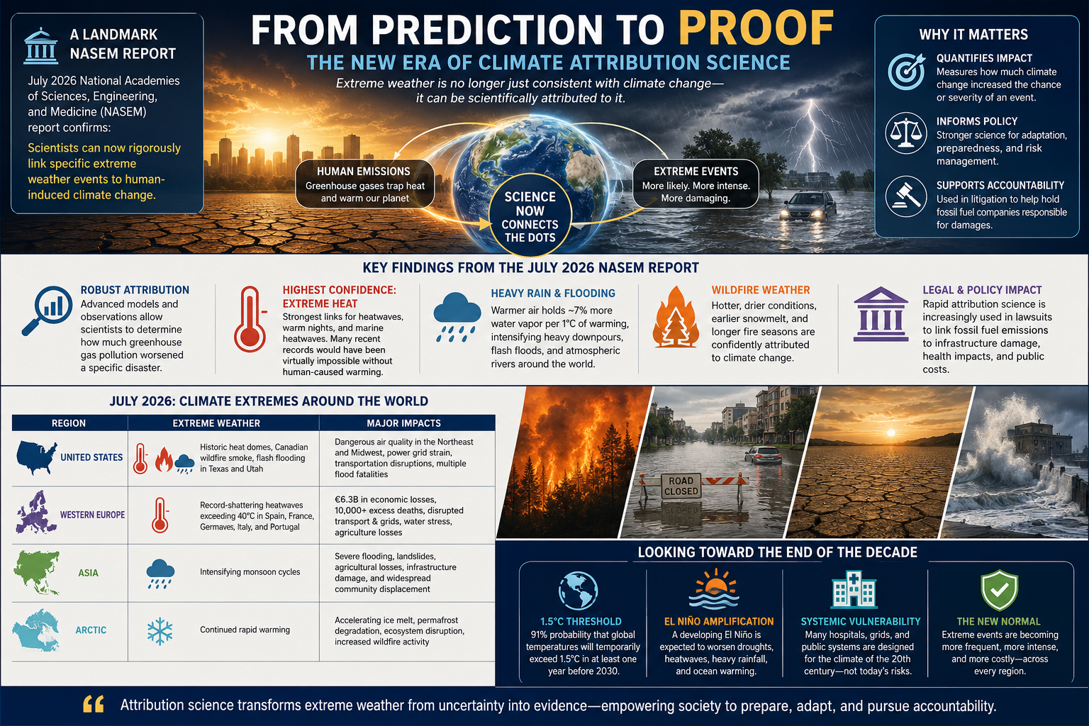
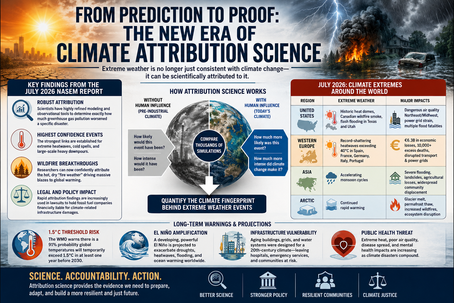
Extreme Weather Is No Longer Just Consistent with Climate Change—It Can Be Scientifically Attributed to It
A landmark 2026 report from the U.S. National Academies of Sciences, Engineering, and Medicine (NASEM) marks a major milestone in climate science. For decades, scientists could say that climate change made extreme weather more likely. Today, the evidence has become substantially stronger: modern attribution science can now determine, with high confidence, how much human-caused climate change increased the probability or severity of many individual extreme weather events.
This represents a profound shift in both science and public policy. Extreme weather is no longer viewed simply as a consequence of natural variability occurring alongside a warming climate. For many classes of events—including record-breaking heatwaves and extreme precipitation—scientists can now quantify the role that greenhouse gas emissions played in producing the disaster.
As climate disasters accelerate across the globe, attribution science is transforming what was once considered “unusual weather” into measurable evidence of a rapidly changing climate system.
A New Scientific Milestone
The July 2026 NASEM report concludes that advances in climate models, observational datasets, satellite measurements, and statistical methods have made attribution science sufficiently mature to evaluate many individual weather disasters with remarkable precision.
Rather than asking whether climate change “caused” a storm, researchers now ask more scientifically meaningful questions:
How much more likely was this event because of global warming?
How much more intense did climate change make the event?
What fraction of the resulting damages can reasonably be attributed to human-caused greenhouse gas emissions?
These questions can now be answered with increasing confidence.
Major Findings of the NASEM Report
Robust Event Attribution
Scientists now possess sophisticated observational records and climate simulations capable of comparing today’s atmosphere with a hypothetical pre-industrial climate.
By running thousands of simulations under both conditions, researchers can estimate how human emissions altered the probability and intensity of an event.
This allows attribution studies to quantify the “climate fingerprint” behind individual disasters.
Highest Confidence: Extreme Heat
The strongest scientific confidence exists for:
prolonged heatwaves
record high temperatures
warm nighttime temperatures
marine heatwaves
Heat events are among the easiest climate signals to detect because rising greenhouse gases directly increase global temperatures.
Many recent record heatwaves would have been virtually impossible without human-caused warming.
Heavy Rainfall and Flooding
Warmer air holds approximately 7% more water vapor for every 1°C of warming, following the Clausius-Clapeyron relationship.
This additional atmospheric moisture increases the likelihood of:
intense rainfall
flash flooding
atmospheric river events
tropical cyclone rainfall
The report concludes that heavy precipitation events now have strong attribution confidence across much of the world.
Wildfire Weather
Although individual wildfires depend upon ignition sources, vegetation, and local weather, researchers can now confidently attribute the hot, dry conditions that create extreme fire weather to climate change.
These include:
prolonged drought
record temperatures
low humidity
earlier snowmelt
longer fire seasons
Climate change may not ignite every fire, but it increasingly creates the environmental conditions that allow fires to spread rapidly and become catastrophic.
Growing Legal Significance
One of the most important implications of attribution science extends beyond meteorology.
Rapid attribution studies are increasingly being introduced into court proceedings involving:
infrastructure damage
insurance losses
municipal adaptation costs
public health impacts
fossil fuel liability
As attribution methods become more rigorous, courts may increasingly rely upon quantitative estimates linking greenhouse gas emissions to specific economic damages.
This development could significantly reshape climate litigation over the coming decades.
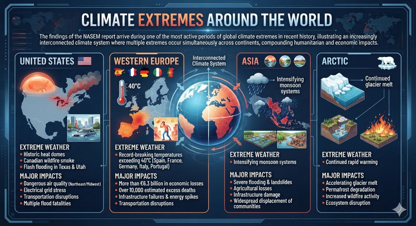
July 2026: Climate Extremes Around the World
The findings of the NASEM report arrive during one of the most active periods of global climate extremes in recent history.
Region
Extreme Weather
Major Impacts
United States
Historic heat domes, Canadian wildfire smoke, flash flooding in Texas and Utah
Dangerous air quality across the Northeast and Midwest, electrical grid stress, transportation disruptions, multiple flood fatalities
Western Europe
Record-breaking temperatures exceeding 40°C across Spain, France, Germany, Italy, and Portugal
More than €6.3 billion in economic losses, over 10,000 estimated excess deaths, infrastructure failures, transportation disruptions, and energy demand spikes
Asia
Intensifying monsoon systems
Severe flooding, landslides, agricultural losses, infrastructure damage, and widespread displacement of communities
These events illustrate an increasingly interconnected climate system in which multiple extremes occur simultaneously across continents, compounding humanitarian and economic impacts.
Looking Toward the End of the Decade
Several independent climate assessments indicate that the world is approaching critical thresholds.
Temporary Exceedance of 1.5°C
The World Meteorological Organization estimates there is approximately a 91% probability that at least one year before 2030 will temporarily exceed 1.5°C above pre-industrial temperatures.
While a single year above 1.5°C does not constitute failure of the Paris Agreement, it demonstrates how rapidly the climate system is approaching thresholds originally expected later in the century.
Developing El Niño
Climate forecasters expect a strengthening El Niño to amplify many existing climate risks, including:
more intense global heat
severe drought in some regions
stronger rainfall elsewhere
increased marine heatwaves
coral bleaching
agricultural disruption
Natural climate variability is increasingly occurring on top of a warmer baseline climate, producing more severe impacts than similar events decades ago.
Infrastructure Built for Yesterday’s Climate
Many public health experts warn that modern infrastructure remains designed around the climate of the twentieth century rather than the rapidly changing conditions of the twenty-first.
Areas of growing concern include:
aging electrical grids
transportation infrastructure
hospitals and emergency care systems
water management systems
cooling capacity in residential buildings
urban heat island effects
As extreme events become more frequent and compound one another, these systems face increasing risks of cascading failures.
The Emerging “New Normal”
The significance of the 2026 NASEM report extends far beyond advances in climate modeling. It reflects a fundamental evolution in how society understands weather disasters.
Scientists are no longer limited to saying that climate change may have influenced an event. Increasingly, they can quantify the extent to which greenhouse gas emissions altered the probability, intensity, and resulting impacts of specific disasters.
This capability strengthens scientific understanding, informs emergency planning, improves risk assessment, supports more resilient infrastructure design, and provides a stronger evidentiary foundation for public policy and legal accountability.
The growing field of event attribution represents a turning point in climate science. As observational records expand and modeling techniques continue to improve, attribution studies will become an increasingly important tool for understanding not only whether climate change is influencing extreme weather, but how much it is contributing to the escalating risks facing societies around the world.
In an era of accelerating climate change, the question is no longer whether human activity is affecting the weather. Increasingly, the scientific challenge is measuring—with ever greater precision—the extent of that influence and using that knowledge to better prepare for the future.
When I began this journey more than three decades ago, I wasn’t a climate researcher. I was a financial planner specializing in business, economics, estate planning, and risk management. My academic background included economics, philosophy, and extensive study in physics, calculus, statistics, and systems analysis. My career focused on a simple question:
How do you create the best possible future for the people who come after you?
In the early 1990s, I met a brilliant scientist named Sidd. We shared a curiosity about complex systems and a desire to test ideas rather than simply debate them. Together, we began an experiment that has now spanned more than thirty years.
Our goal was unusual. We wanted to build what we jokingly called a one-size-fits-all, bulletproof shareware estate plan—not for one family, but for every family on Earth.
At the same time, I was helping pioneer some of the earliest privately owned web servers. Before commercial hosting became commonplace, we were operating online while many organizations were still connected through universities. It was the same era when Yahoo! itself was running from Stanford University.
By 1995, our website, KingArthur.com, was attracting millions of visitors each month. The internet gave us something few researchers had ever possessed: the ability to interact directly with millions of people across cultures, countries, religions, and generations.
One question became central to our experiment:
“When it comes to your life and what you leave behind, what is the single most important thing?”
We expected many people to answer with wealth, success, fame, or legacy.
Instead, they overwhelmingly answered something much simpler.
Among people under fifty, the most common answer was their children.
Among those over fifty, the answer shifted to their grandchildren.
The experiment revealed something profound. The greatest wealth most people hope to preserve is not money. It is the opportunity for future generations to experience the same joys they have experienced themselves.
In other words, the ultimate estate plan is remarkably simple:
To my children’s children’s children.
The greatest inheritance most of us hope to leave is not a larger bank account. It is the chance for our descendants to raise children of their own, watch them grow, and someday become grandparents themselves.
When we began this experiment, I did not have grandchildren.
Today I do.
That changes everything.
Coincidentally, I was recently asked a question that perfectly captured the purpose of this work:
“Can you play with me on this? I’m wearing my nutritional ecologist hat here, and I’m in a municipal-level discussion that is trying to zoom out seven generations while also identifying the baby steps needed over the next four-year election cycle.”
My immediate thought was:
Exactly.
That is what this experiment has always been about.
An estate plan should not end with our children—or even our grandchildren. It should extend seven generations into the future.
My grandchildren deserve the opportunity to become grandparents themselves. Their grandchildren deserve the same opportunity.
That is entirely achievable—but only if we make wise decisions today.
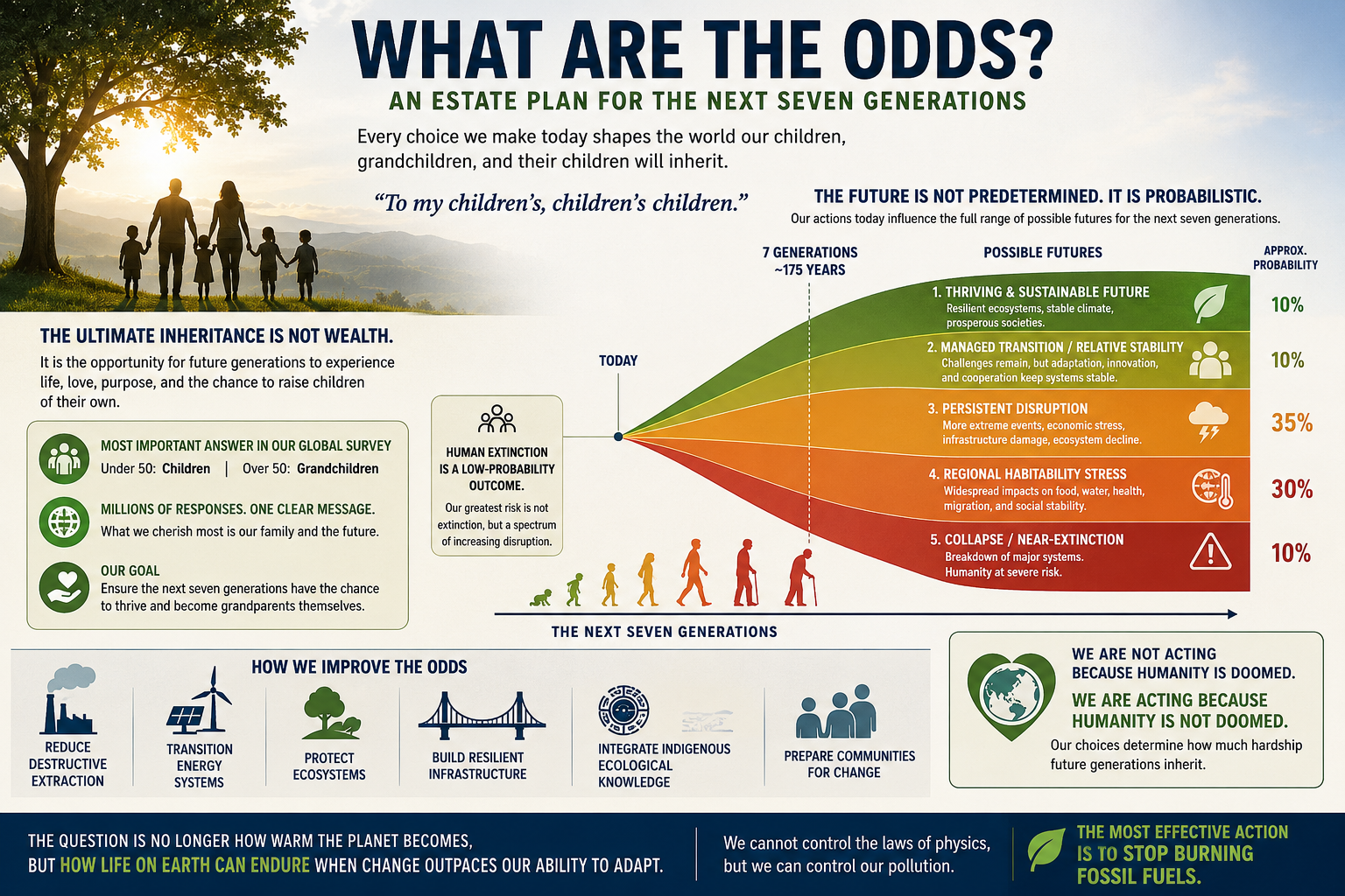
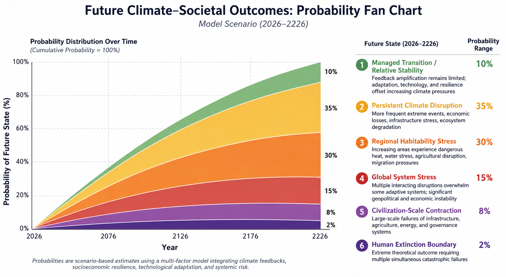
The graph that follows illustrates that idea.
Every choice we make now influences the range of possible futures available to the next seven generations.
Some outcomes are relatively optimistic. Some involve increasing climate disruption.
Some are far more severe.
Importantly, human extinction remains a low-probability outcome.
The far more likely future is not one of sudden extinction, but one that spans a spectrum of increasing disruption—affecting ecosystems, agriculture, infrastructure, economies, public health, migration, and regional habitability.
The probabilities are not fixed. They are shaped by the decisions humanity makes over the coming decades.. including today.
That changes the conversation entirely.
The question is no longer:
“Are humans going extinct?”
The more important question is:
“How difficult do we want life to be for the next seven generations?”
That question naturally leads to practical priorities:
Reduce destructive extraction of fossil fuels and natural resources.
Transition to cleaner and more resilient energy systems.
Protect and restore forests, wetlands, and other ecosystems.
Build infrastructure capable of withstanding future climate conditions.
Integrate Indigenous ecological knowledge alongside modern science.
Prepare communities to adapt to unavoidable change.
The most important message is this:
We are not acting because humanity is doomed.
We are acting because humanity is not doomed.
Our choices today determine how much hardship future generations inherit.
Ultimately, this is not simply a discussion about climate change.
It is an estate planning exercise on a planetary scale.
The question is no longer how warm the planet becomes.
The question is how well civilization—and the generations that follow us—can endure as environmental change accelerates faster than our ability to adapt.
We cannot rewrite the laws of physics. But we can decide how much pollution we continue to add to the atmosphere.
The most effective step we can take is also the simplest:
Stop burning fossil fuels as quickly and responsibly as possible, while building a more resilient world for the generations that follow.
The probability envelope broadens because uncertainty increases as multiple systems interact.
Period 4: 2200–2226
Long-Term Equilibrium Selection
Possible pathways:
Pathway A: Adapted Earth System
Outcome:
Stable but transformed civilization
Pathway B: High-Stress Earth System
Outcome:
Persistent disruption and regional instability
Pathway C: Cascading Failure
Outcome:
Civilization contraction
The Framework’s Core Equation
A simplified representation:
Interpretation of the Upper Boundary
The framework separates:
Planetary Habitability
from:
Human Civilization
The probability hierarchy is:
The model therefore treats human extinction as a low-probability upper boundary, not the central pathway.
The more probable outcome under increasing nonlinear acceleration is:
A progressively more difficult Earth for existing human systems to operate within.
Sensitivity Analysis
The largest factors shifting the probability envelope would be:
Variable
Effect
Feedback coupling increases
Moves probability toward disruption
Acceleration increases
Compresses response time
Ecosystem degradation increases
Raises vulnerability
Adaptation improves
Moves probability toward stability
Resilience declines
Raises systemic risk
Feedbacks weaken
Moves probability toward stabilization
Summary Distribution
The theoretical 200-year envelope:
Most Probable Region:

Persistent Disruption
        ↓
Regional Habitability Stress


Less Probable:

Global System Stress
        ↓
Civilization Contraction


Extreme Upper Boundary:

Human Extinction
Framework Conclusion
Under the Nonlinear Acceleration Framework, the primary risk is not a sudden transition from a habitable Earth to an uninhabitable planet.
The dominant theoretical risk pathway is:
Increasing Feedback Coupling → Accelerating Impacts → Reduced Recovery Time → Growing System Stress → Progressive Civilization Challenges
The extinction boundary exists as the extreme edge of the probability envelope, while the central concern is the increasing probability of a world where human systems must operate under rapidly changing environmental conditions.
Understanding Climate Change as a Cascading System
A Public Access Explanation of Feedbacks, Acceleration, and Future Pathways
A Probability Distribution of Humanity’s Next 200 Years
How likely are different futures for civilization as climate change accelerates?
Here is a Climate-Societal Probability Fan Chart (2026–2226) that visualizes a model-based distribution of potential outcomes over the next two centuries.
Rather than asking “What will happen?”, the chart asks the more scientifically useful question:
“What is the probability distribution of plausible futures?”
The model incorporates nonlinear climate feedbacks, systemic interactions, adaptive capacity, technological progress, and societal resilience to estimate the relative likelihood of six broad scenarios:
The important takeaway is that human extinction is not the central expectation of the model. The highest-probability outcomes involve increasing disruption, economic stress, migration, infrastructure challenges, and declining habitability across vulnerable regions—not the disappearance of humanity.
Understanding probability distributions is far more informative than focusing on a single prediction. As with weather forecasting or hurricane models, uncertainty is not ignorance—it is measurable.
Our goal is to move the conversation beyond sensationalism and toward evidence-based risk assessment grounded in systems science, nonlinear feedbacks, and probability.
Discussion and constructive criticism are welcome.
Introduction
Climate change is often described as a simple process:
More greenhouse gases → Higher temperatures → More impacts
This explanation captures an important part of the process, but it does not fully describe how complex systems behave.
The Earth is not a machine with separate parts operating independently.
It is a connected system where:
Atmosphere ↔ Oceans ↔ Ice Systems ↔ Ecosystems ↔ Human Civilization
When one part changes, other parts respond.
Sometimes those responses reduce change.
Sometimes they amplify it.
The Nonlinear Acceleration Framework explores how connected responses can transform climate change from a gradual process into a system of interacting feedbacks.
1. The Earth Is a Connected System
The Earth operates as an interconnected network.
Changes do not remain isolated.
A disturbance in one system can propagate into another:
Atmosphere → Ocean → Cryosphere → Biosphere → Human Systems
A Theoretical Model of Coupled Feedback Amplification, System-State Transitions, and Future Climate Trajectories
Abstract
Climate change is often represented as a sequence of approximately linear responses to increasing radiative forcing. However, complex Earth systems do not evolve as isolated variables responding independently to external perturbations. They behave as interconnected nonlinear systems in which feedback interactions can amplify, redistribute, and accelerate responses over time.
This paper presents a theoretical framework—the Nonlinear Acceleration Framework (NAF)—for describing climate evolution as a coupled dynamical system governed by interacting physical, ecological, and societal processes. The framework proposes that climate impacts should not be evaluated solely through individual trends but through the changing acceleration of interconnected system variables.
The central hypothesis is that the Earth system can experience emergent nonlinear acceleration when multiple feedback mechanisms become coupled. In this formulation, relatively small perturbations may propagate through interconnected subsystems, creating cascading responses analogous to network failures in other complex systems.
The paper introduces a conceptual probability envelope rather than a deterministic prediction. The envelope represents a range of possible future trajectories, extending from relative climate stabilization through increasing disruption, regional habitability loss, civilization-scale stress, and theoretical upper-bound outcomes involving human extinction. These pathways are constrained by fundamental physical principles, including conservation of energy, radiative transfer, thermodynamics, ocean heat capacity, atmospheric moisture relationships, and nonlinear dynamical behavior.
The framework does not claim that extreme outcomes are inevitable. Rather, it proposes that increasing coupling among climate subsystems may shift probability distributions away from stable states and toward progressively more disruptive states.
This theoretical model provides a foundation for future mathematical development through stochastic dynamical systems, Bayesian inference, and computational simulations.
The Earth’s climate system is not a collection of independent components. It is a coupled network consisting of interacting physical, chemical, biological, and human systems. The atmosphere, oceans, cryosphere, biosphere, and human infrastructure exchange energy and information continuously.
Traditional approaches often analyze climate impacts through individual variables:
atmospheric temperature,
ocean heat content,
sea-level rise,
precipitation patterns,
ecosystem responses.
While these measurements remain essential, a complex systems perspective suggests that the behavior of the whole system cannot always be inferred from isolated components.
A defining characteristic of complex nonlinear systems is that the response of the system may not be proportional to the initial disturbance.
A small perturbation can:
activate feedback mechanisms,
alter system conditions,
increase the probability of additional responses,
create interactions among previously separated processes.
This behavior is commonly described as emergence.
The central premise of the Nonlinear Acceleration Framework is that climate change should be evaluated not only by the magnitude of change, but by the changing rate of change and the increasing interaction among feedback pathways.
A linear interpretation assumes:Change∝Forcing
A nonlinear interpretation considers:
where the evolution of the system depends not only on external forcing but also on the internal state of the system itself.
In this formulation, the climate system can move through different dynamical regimes.
A relatively stable regime may transition into:
increasing variability,
amplified extremes,
cascading feedback activation,
regional system failures,
broader societal disruption.
The purpose of this paper is to establish a theoretical structure for describing these transitions.
The framework is built around three concepts:
1. Nonlinear Acceleration
The rate of change of climate variables may itself change over time.
2. The Domino Effect
Individual feedback mechanisms may become connected, allowing disturbances to propagate through the Earth system.
3. Probability Envelopes
Future outcomes should be represented as distributions of possible trajectories rather than single deterministic forecasts.
2. Foundations of the Nonlinear Acceleration Framework
2.1 Climate as a Complex Adaptive System
A complex adaptive system contains:
multiple interacting components,
feedback loops,
thresholds,
nonlinear responses,
emergent behavior.
The climate system satisfies these characteristics.
Represent the Earth system as:
where:
A = atmosphere
O = ocean system
C = cryosphere
B = biosphere
H = human systems
The evolution of the system is:
where:
F represents internal system dynamics,
E represents external forcing.
The critical insight is that:
The system itself changes as conditions evolve.
A warmer ocean is not simply the same ocean at a higher temperature. It has altered:
circulation patterns,
evaporation rates,
atmospheric moisture content,
biological conditions,
ice interactions.
The system state modifies future evolution.
2.2 Acceleration as a Primary Variable
Most analyses focus on:
the value of a climate variable.
The Nonlinear Acceleration Framework introduces a second-order perspective:
and:
The first derivative represents the rate of change.
The second derivative represents acceleration.
A system undergoing acceleration behaves differently from a system experiencing constant change.
For example:
Linear:
Accelerating:
where:
k represents the growth constant.
The doubling time is:
A declining doubling time indicates increasing acceleration.
The framework proposes that coupled climate indicators can be evaluated through changing characteristic timescales.
2.3 Coupled Feedback Dynamics
A feedback loop occurs when a change in one component influences another component, which then feeds back into the original component.
A simplified example:
The initial disturbance becomes amplified.
The feedback gain can be represented as:
where each:
represents the influence of an individual feedback process.
If:
the disturbance tends to decay.
If:
the disturbance tends to amplify.
The theoretical concern of nonlinear acceleration is not the existence of individual feedbacks, but the possibility that multiple feedbacks become increasingly coupled.
3. Physical Constraints on Climate Evolution
A theoretical framework must remain bounded by fundamental physical laws.
Nonlinear acceleration does not imply unlimited warming.
The Earth system operates within physical constraints.
3.1 Conservation of Energy
The climate system follows energy conservation:
Incoming solar radiation must balance outgoing radiation over time.
Changes in greenhouse gas concentrations alter the balance between incoming and outgoing energy.
However, the resulting temperature response remains constrained by:
atmospheric composition,
ocean heat storage,
surface properties,
feedback strength.
3.2 Radiative Equilibrium
The Earth emits infrared radiation according to temperature.
A simplified representation:
where:
F is emitted radiation,
σ is the Stefan-Boltzmann constant,
T is temperature.
Increasing atmospheric absorption changes the effective emission level and requires adjustment toward a new equilibrium.
The equilibrium response is not instantaneous because different components respond at different timescales.
3.3 Ocean Heat Capacity
The oceans represent a massive thermal reservoir.
The temperature response can be represented as:
where:
m is mass,
c is heat capacity,
ΔT is temperature change.
Because oceans store enormous quantities of heat, they moderate short-term atmospheric responses.
However, stored heat also represents delayed energy release into the climate system.
3.4 Atmospheric Moisture Amplification
Atmospheric water vapor is a major climate feedback because warmer air can contain more moisture.
The relationship is nonlinear and follows thermodynamic constraints.
A warmer atmosphere increases:
moisture capacity,
latent heat transport,
potential precipitation intensity.
This creates additional coupling between:
temperature,
humidity,
storms,
flooding,
and atmospheric circulation.
3.5 Physical Limits and Upper Boundaries
A critical distinction must be made between:
Earth-system destabilization
and
planetary runaway warming.
A nonlinear climate trajectory does not imply conditions comparable to Venus.
The theoretical upper boundary considered here is therefore not unlimited temperature increase, but progressive degradation of conditions required for complex human civilization.
The relevant question becomes:
Not:
“Can Earth become Venus?”
but:
“What range of Earth conditions remains compatible with current human systems?”
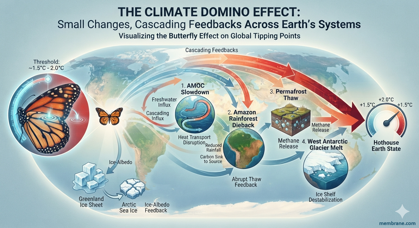
4. The Domino Effect:
Climate Feedbacks as a Coupled Nonlinear Network
The central premise of the Nonlinear Acceleration Framework is that climate change cannot be adequately represented as a collection of independent trends. The Earth system operates as a network of interacting processes where disturbances can propagate across multiple domains.
This section introduces the Domino Effect hypothesis: the possibility that a perturbation in one subsystem can increase the probability of changes in connected subsystems, producing a cascade of reinforcing responses.
The metaphor of falling dominoes is not intended to imply a predetermined sequence. Rather, it describes a network effect in which the state change of one component modifies the conditions of neighboring components.
In mathematical terms, the climate system can be represented as a directed graph:
where:
V represents climate, ecological, and societal components,
E represents the interactions between components.
Each node contains a state variable:
and each connection contains an influence coefficient:
where:
represents how changes in one system influence another.
The complete system becomes:
The important property of this formulation is that the behavior of one component depends on the state of the entire network.
4.1 From Individual Feedbacks to Feedback Networks
Individual feedback mechanisms are often examined separately.
Examples include:
or:
or:
However, nonlinear behavior emerges when these pathways interact.
The effect of a single feedback can be represented as:
The combined effect of multiple interacting feedbacks can be represented by:
The first term represents independent feedbacks.
The second term represents interaction effects.
The critical theoretical proposition is that:
may become increasingly important as coupling increases.
This represents the transition from:
a system containing feedbacks
to:
a feedback-dominated system.
4.3 Cascading Transitions
Complex systems often experience transitions when internal connections exceed stabilizing forces.
Define:
When:
the system tends toward recovery.
When:
the system becomes highly sensitive.
When:
amplifying processes dominate.
This does not mean collapse is guaranteed.
It means the probability distribution of future states shifts.
A small disturbance occurring in a weakly coupled system may disappear.
The same disturbance occurring in a highly coupled system may propagate.
4.4 Examples of Domino-Style Interactions
Cryosphere Pathway
A simplified pathway:TemperatureIncrease
↓IceReduction
↓SurfaceReflectivityChange
↓AdditionalEnergyAbsorption
↓FurtherWarming
The initial disturbance is amplified through a secondary pathway.
Ocean-Atmosphere Pathway
OceanHeating
↓IncreasedEvaporation
↓AtmosphericMoistureIncrease
↓ChangedPrecipitationExtremes
↓Flooding/Drought Variability
↓EcosystemandInfrastructureStress
Biosphere Pathway
HeatStress
↓VegetationLoss
↓CarbonCycleAlteration
↓ReducedNaturalBufferingCapacity
↓AdditionalAtmosphericChanges
5. State-Space Representation of Earth-System Trajectories
A major limitation of simple forecasting is that it attempts to estimate a single future value.
Complex systems do not evolve along a single predictable path.
Instead, they occupy a region of possible states.
5.1 Defining the Climate State Vector
The Earth system can be represented as:
where:
C = cryosphere state
O = ocean state
A = atmosphere state
B = biosphere state
H = human system state
Each component contains multiple variables.
For example:O=HeatCirculationChemistryBiology
The complete Earth system exists as a point in a multidimensional phase space.
5.2 Climate Trajectories
The evolution of the system becomes:
where:
F represents system dynamics,
U(t) represents external forcing,
ϵ represents stochastic variability.
The future is therefore not a single line.
It is a collection of possible trajectories:
5.3 Stability Regions
Complex systems often contain regions called attractors.
An attractor represents a range of states toward which the system tends to evolve.
A simplified representation:
          Stable Region

              ●


       Increasing Instability


              ●


       High Stress Region


              ●


       System Transformation
The theoretical question becomes:
How does increasing nonlinear coupling affect the movement of the system between regions?
5.4 Threshold Dynamics
Thresholds occur when gradual changes produce abrupt responses.
Mathematically:
may produce gradual change.
But:
may produce a nonlinear transition.
The framework treats thresholds not as isolated points but as interacting boundaries.
A single threshold crossing may alter the probability of crossing other thresholds.
6. The Conceptual Probability Envelope
6.1 Purpose
The purpose of the probability envelope is not to produce a single prediction.
Instead, it describes how the distribution of possible futures may shift as nonlinear coupling changes.
The framework defines future states as:
where possible states include:
relative stability,
increasing disruption,
regional habitability loss,
systemic civilization stress,
civilization collapse,
theoretical extinction boundary.
6.2 Probability Distribution
The probability of each state is:
where:
Si represents a future state,
F represents the combined feedback condition.
The probability distribution must satisfy:
As nonlinear coupling increases, the distribution may shift:
Early State:

Stability
█████████

Disruption
██

Collapse
█

Extinction
.


Later State:

Stability
███

Disruption
███████

Collapse
████

Extinction
█
The framework does not state that the upper outcomes are inevitable.
It states that increasing system coupling changes the shape of the probability landscape.
6.3 Scenario Categories
The conceptual envelope contains six broad regions.
Scenario 1:
Relative Stabilization
Characteristics:
feedback amplification remains limited,
adaptation remains effective,
system coupling remains manageable.
State:
Scenario 2:
Increasing Climate Disruption
Characteristics:
increasing extreme events,
infrastructure stress,
economic impacts.
State:
Scenario 3:
Regional Habitability Stress
Characteristics:
increasing areas experiencing dangerous conditions,
agricultural disruption,
migration pressures.
State:
Scenario 4:
Global System Stress
Characteristics:
multiple simultaneous disruptions,
declining adaptive capacity,
interconnected failures.
State:
Scenario 5:
Civilization-Scale Contraction
Characteristics:
severe loss of infrastructure reliability,
economic fragmentation,
reduced technological capacity.
State:
Scenario 6:
Human Extinction Boundary
Characteristics:
extreme theoretical conditions,
failure of global adaptation,
loss of environments capable of sustaining human populations.
State:
This represents an upper-bound possibility, not a prediction.
6.4 Interpretation
The central conclusion of the probability envelope is:
The most important variable is not only the amount of climate change, but the degree of coupling among interacting systems.
A world with large individual changes but weak coupling may remain manageable.
A world with moderate changes and strong coupling may experience cascading effects.
The framework therefore shifts the question from:
“How much warming occurs?”
to:
“How does the Earth system respond as connections among components intensify?”
7. Mathematical Development of the Nonlinear Probability Model
7.1 From Conceptual Framework to Dynamical Model
The previous sections described the Earth system as a coupled nonlinear network. This section develops a mathematical structure for representing the evolution of possible future states.
The purpose of this model is not to claim a deterministic forecast. Instead, it provides a mathematical language for describing how changes in feedback strength, coupling, and system resilience could alter the distribution of possible trajectories.
The general form of a nonlinear dynamical system is:
where:
X is the Earth-system state vector,
F(X,t) represents deterministic system behavior,
η(t) represents stochastic variability.
The inclusion of η(t) recognizes that complex systems are influenced by internal variability and unpredictable perturbations.
The system therefore evolves through both:
deterministic physical processes,
probabilistic events.
7.2 The Nonlinear Acceleration State Vector
The Nonlinear Acceleration Framework proposes that important indicators should not be evaluated only by their magnitude but also by their rate of change.
The extinction boundary represents the extreme upper limit of the probability envelope, not the expected trajectory.
8.3 The Role of Adaptation
The probability envelope is not controlled only by physical processes.
Human systems are also dynamic.
Adaptation modifies:
the societal resilience component.
A more resilient society may remain within lower disruption states despite increased climate stress.
A less resilient society may transition more rapidly between states.
The framework therefore includes human response as an internal variable rather than treating civilization as a passive observer.
8.4 Implications of the Framework
The theoretical implications are:
Climate risks should be evaluated as interacting networks rather than isolated events.
Acceleration may be as important as magnitude.
Feedback coupling may alter the distribution of possible futures.
Future outcomes should be represented as probability landscapes rather than single predictions.
The most consequential transitions may occur through cascading interactions rather than individual events.
9. Limitations of the Framework
A theoretical framework must clearly define what it does and does not establish.
9.1 Parameter Uncertainty
The coupling coefficients:
are not yet empirically determined.
Future work must estimate these values through observations and simulations.
9.2 Model Dependence
Probability outputs from this framework would depend on:
initial assumptions,
selected variables,
weighting functions,
feedback representation.
Different assumptions may produce different probability distributions.
9.3 Complexity Limits
Earth systems contain enormous complexity.
No mathematical model can perfectly represent every interaction.
The purpose of the framework is therefore not prediction perfection but improved representation of nonlinear relationships.
9.4 Validation Requirement
A future computational implementation would require:
historical testing,
comparison against observed system behavior,
uncertainty analysis,
sensitivity testing.
Only after such testing could numerical probability estimates be evaluated.
10. Conclusions
The Nonlinear Acceleration Framework presents a theoretical approach for understanding climate evolution as a nonlinear coupled system rather than a collection of independent trends.
The central hypothesis is that the most important feature of future climate dynamics may not be the magnitude of individual changes, but the increasing interaction among those changes.
Through the Domino Effect concept, climate feedbacks are represented as interconnected pathways capable of amplifying disturbances.
Through state-space modeling, possible futures are represented as trajectories rather than a single deterministic forecast.
Through the probability envelope concept, outcomes are represented as a continuously shifting distribution ranging from manageable disruption to increasingly severe system states.
The framework does not establish that extreme outcomes are inevitable.
Rather, it proposes that as nonlinear coupling increases, the structure of possible futures changes.
The fundamental research question becomes:
How does the probability distribution of Earth-system outcomes evolve as feedback interactions, acceleration rates, and system coupling change?
Answering that question requires further mathematical development, computational simulation, and empirical evaluation.
The purpose of this theoretical framework is to provide a foundation for that investigation.
Appendix A
Mathematical Formulation Summary
Earth-System Dynamics
Coupled System
Acceleration
Domino Amplification
Collapse Index
Probability Evolution
Appendix B
Proposed Computational Implementation
A future numerical model could proceed through:
Step 1
Define system variables:
Step 2
Estimate coupling relationships:
Step 3
Generate stochastic trajectories:
Step 4
Calculate:
Collapse Index
Transition probabilities
State occupancy
Step 5
Produce probability envelope:
Probability Density

 ^
 |
 |        Current
 |          |
 |          V
 |
 |       _______
 |      /       \
 |_____/         \_____________

 Stability   Disruption   Collapse

              Future State →
Final Statement
The Nonlinear Acceleration Framework is best understood as a proposed complex-systems model of climate evolution. Its central contribution is the integration of acceleration, feedback coupling, network effects, and probability distributions into a unified theoretical structure.
The framework transforms the question from:
“What will happen at a given temperature?”
to:
“How does a changing nonlinear Earth system reshape the probability landscape of possible futures?”
This question represents the foundation for future mathematical and computational investigation.
Addendum
Extending the Nonlinear Acceleration Framework:
A Formal Bayesian-Stochastic Implementation of the Climate Probability Envelope
Abstract
This addendum extends the theoretical Nonlinear Acceleration Framework (NAF) by proposing a formal mathematical pathway for converting the conceptual probability envelope into a stochastic dynamical model.
The original framework defines climate change as a nonlinear coupled system in which interacting physical, ecological, and societal processes can modify the probability distribution of future states. This extension introduces a computational architecture based on:
nonlinear dynamical systems,
Bayesian probability updating,
stochastic differential equations,
network coupling analysis,
Monte Carlo trajectory sampling.
The purpose of this model is not to generate predetermined forecasts, but to establish a mathematical framework capable of exploring how assumptions about feedback strength, coupling, resilience, and adaptation influence future trajectories.
The model treats future climate outcomes as a probability distribution evolving through time rather than as a single deterministic pathway.
1. Introduction
The previous framework established three fundamental concepts:
Nonlinear Acceleration The possibility that rates of change may themselves increase.
The Domino Effect The possibility that interactions among subsystems amplify disturbances.
The Probability Envelope The concept that future states exist as a distribution of possible outcomes rather than a single trajectory.
The next step is to construct a mathematical representation capable of simulating these concepts.
The proposed model treats the Earth system as a stochastic nonlinear network.
The general form is:
where:
X = system state vector,
f = nonlinear deterministic dynamics,
θ = model parameters,
Σ = stochastic variability function,
Wt = stochastic process.
The model therefore contains both:
predictable physical relationships,
unpredictable variability.
2. Defining the Earth-System State Vector
The system is represented by:
where:
Variable
Meaning
O
Ocean thermal state
C
Cryosphere state
A
Atmospheric state
B
Biosphere state
H
Human-system stress
R
Resilience/adaptation capacity
2.1 Ocean State
The ocean component includes:
where:
OHC = ocean heat content,
MHW = marine heatwave intensity,
CIRC = circulation state.
2.2 Cryosphere State
where:
ice loss,
surface reflectivity,
frozen carbon systems
are represented as interacting variables.
2.3 Atmospheric State
where:
T=temperature,
V=water vapor,
P=precipitation extremes,
E=extreme weather intensity.
2.4 Biosphere State
2.5 Human-System State
2.6 Resilience State
This component is essential because human outcomes are not determined by climate physics alone.
3. The Coupled Feedback Matrix
The Earth system is represented as a network:
The diagonal terms represent internal behavior.
The off-diagonal terms represent coupling.
For example:
represents ocean influence on cryosphere.
represents cryosphere influence on atmosphere.
represents biosphere influence on human systems.
4. The Nonlinear Acceleration Operator
Traditional models evaluate:
The NAF evaluates:
and:
Define the acceleration operator:
The system acceleration state becomes:
where:
low As indicates stable evolution,
high As indicates accelerating transition.
5. Bayesian Probability Architecture
The model defines possible future states:
where:
State
Description
S1
Relative stabilization
S2
Increasing disruption
S3
Regional habitability stress
S4
Global systemic stress
S5
Civilization-scale contraction
S6
Human extinction boundary
5.1 Prior Distribution
Initial assumptions:
represent the starting probability distribution.
The model does not assume fixed values.
They are parameters.
5.2 Evidence Updating
New system information modifies the distribution:
where:
represents the evolving system indicators.
6. Monte Carlo Probability Envelope
The model generates thousands or millions of possible trajectories.
Each simulation samples:
feedback strength,
coupling coefficients,
stochastic variability,
resilience parameters.
Example:
may represent a high-resilience pathway.
may represent a low-resilience pathway.
After many simulations:
produce a distribution.
7. Example Model Output Structure
The output is not:
“The probability of collapse is exactly X%.”
Instead:
“Under assumptions A through Z, the simulated probability distribution occupies the following regions.”
Example:
Outcome
Model Scenario Range
Relative stabilization
5–20%
Persistent disruption
25–50%
Regional system stress
20–40%
Civilization-scale stress
5–25%
Extinction boundary
<5%
These values are illustrative placeholders demonstrating the model structure, not empirical predictions.
8. Sensitivity Analysis
The model’s most important function may be identifying which assumptions dominate outcomes.
A sensitivity function:
measures how much changing parameter θi affects the probability distribution.
Possible sensitivity variables:
feedback coupling,
adaptation capacity,
ecosystem resilience,
ocean buffering,
infrastructure vulnerability.
9. Emergent Behavior and Phase Transitions
A central hypothesis is that the probability distribution may shift nonlinearly.
Small parameter changes may produce large outcome changes.
Mathematically:
near transition zones.
This represents a possible phase transition.
10. Research Program
A complete implementation would require:
Phase 1
Define variables and coupling relationships.
Phase 2
Construct computational simulations.
Phase 3
Compare model behavior against historical system evolution.
Phase 4
Perform uncertainty analysis.
Phase 5
Evaluate predictive skill.
11. Final Synthesis
The Nonlinear Acceleration Framework proposes that climate change should be understood as a transition within a complex adaptive system.
The key concepts are:
Instead:
The Domino Effect explains how disturbances propagate.
The acceleration framework explains how rates of change may evolve.
The probability envelope explains how future states exist as a distribution rather than a single path.
The Bayesian-stochastic extension provides a pathway for transforming these concepts into a computational model.
The ultimate scientific question becomes:How does increasing system coupling reshape the probability landscape of Earth−system futures?
The answer requires continued mathematical development, computational testing, and empirical evaluation.
This addendum provides the theoretical architecture for that next stage.
Addendum II
The Nonlinear Acceleration Framework:
A Network-Based Catastrophe Theory Extension and Computational Architecture for Coupled Earth-System Transitions
Abstract
This addendum extends the Nonlinear Acceleration Framework (NAF) by introducing a network-based catastrophe theory approach for analyzing how coupled Earth-system processes may transition between relatively stable and increasingly disrupted states.
The central hypothesis explored here is that climate-system evolution is not governed only by the magnitude of external forcing, but also by the internal connectivity, feedback strength, and resilience characteristics of the system.
A complex network may remain stable while individual disturbances are absorbed. However, as coupling strength increases, the system may approach critical transition regions where small perturbations generate disproportionately large responses.
This extension introduces:
a climate feedback network model,
a critical connectivity threshold,
resilience-collapse dynamics,
phase-transition behavior,
early-warning indicators,
a computational architecture for future simulations.
The framework does not define deterministic outcomes. Instead, it proposes a mathematical method for exploring how the probability distribution of possible futures changes as system properties evolve.
1. Introduction:
From Feedback Loops to Network Dynamics
The traditional representation of climate feedbacks often focuses on individual mechanisms.
Examples:
or:
These pathways are important, but complex systems rarely operate through isolated chains.
A network perspective recognizes that:
multiple feedbacks operate simultaneously,
feedback strengths change over time,
interactions create emergent properties,
system behavior depends on connectivity.
The Earth system can therefore be represented as:
where:
V = system components,
E = connections,
W = connection strengths.
The behavior of the whole system emerges from the structure of the network.
2. Climate Network Representation
2.1 Nodes
The network consists of interacting nodes:
Each node contains internal variables.
For example:Ocean={Heat,Circulation,Chemistry,Biology}
2.2 Edges
Connections represent influence:
Examples:
through evaporation.
through albedo effects.
through carbon exchange.
2.3 Weighted Coupling
Each connection has strength:
The total network influence is:
The hypothesis is:
Increasing total coupling can increase the probability of nonlinear system transitions.
3. Network Criticality
Complex networks often experience transitions when connectivity increases beyond a critical level.
Define:
where:
represents network connectivity.
Low Connectivity State
Characteristics:
disturbances remain localized,
feedbacks remain limited,
recovery mechanisms dominate.
Critical Connectivity State
Characteristics:
increased variability,
slower recovery,
greater sensitivity.
High Connectivity State
Characteristics:
disturbances propagate,
feedback interactions dominate,
system becomes more nonlinear.
4. Resilience as a Competing Force
A central component of the framework is that amplification and stabilization operate simultaneously.
Define:
as system resilience.
Define:
as amplification force.
The transition condition becomes:
When:
the system tends toward stabilization.
When:
the system becomes highly sensitive.
When:
transition probability increases.
5. Catastrophe Theory Representation
Catastrophe theory studies systems where gradual changes can produce abrupt transitions.
A simplified potential function:
describes the stability landscape.
The system moves toward minimum-energy states:
A changing climate system modifies the landscape itself.
The valleys representing stable states may become shallower.
The barriers separating states may decrease.
Example:
Stable climate state:
        ______
       /      \
______/        \______
Increasing instability:
      __
_____/  \_____
Transition:
____          ____
    \________/
The system moves into a different state region.
6. Early Warning Indicators
A nonlinear system approaching transition may exhibit characteristic behaviors.
6.1 Increased Variability
The variance increases:
6.2 Slower Recovery
Recovery time increases:
6.3 Increased Synchronization
Previously separate systems become correlated:
6.4 Increased Autocorrelation
The system retains memory:
These indicators represent theoretical diagnostic tools.
7. Coupled Human-Earth System Dynamics
A major extension of the framework is treating human civilization as part of the system.
The human system is not external.
It both influences and responds to climate conditions.
Define:
as societal capacity.
Then:
where:
A = adaptation capacity,
Hs = accumulated stress.
Positive Human Feedback
Example:
Negative Human Feedback
Example:
The future trajectory depends on which feedback dominates.
8. Civilization Resilience Index
Define:
Interpretation:
Adaptation exceeds stress.
Critical balance.
Stress exceeds adaptation.
The index interacts with the climate Collapse Index:
9. Multi-Dimensional Probability Envelope
The original probability envelope becomes a multidimensional surface.
Instead of:
we define:
The probability landscape changes as:
physical conditions change,
network connectivity changes,
human response changes.
10. Computational Experiment Design
A future simulation could proceed:
Step 1
Initialize Earth-system network.
Step 2
Assign coupling strengths.
Step 3
Introduce perturbations.
Examples:
temperature forcing,
ecosystem disturbance,
infrastructure stress.
Step 4
Run trajectories:
Step 5
Measure:
transition frequency,
resilience,
probability distribution shifts.
11. Research Questions Generated by the Framework
This extension produces several testable questions:
Question 1
Does increasing climate-system coupling produce measurable changes in variance and recovery time?
Question 2
Can network connectivity metrics improve understanding of compound climate events?
Question 3
How does adaptation capacity modify transition probabilities?
Question 4
Are climate impacts better represented as independent events or network cascades?
12. Conclusion
The Network Catastrophe Theory extension expands the Nonlinear Acceleration Framework from a collection of feedback relationships into a coupled dynamical architecture.
The central hypothesis is:
Instead:
The most consequential changes may emerge not from any single component, but from interactions among components.
The framework therefore proposes a new analytical perspective:
Climate change is not only a problem of increasing averages.
It is a problem of changing system dynamics.
The future Earth system may be understood as a probability landscape shaped by:
physical forcing,
nonlinear feedbacks,
network connectivity,
resilience,
and human adaptation.
The next stage of development is the construction of computational models capable of testing these theoretical relationships.
Addendum III
The Nonlinear Acceleration Index (NAI):
A Quantitative Metric for Measuring Climate-System Acceleration, Coupling, and Transition Risk
Purpose: Convert the conceptual framework into measurable indices.
Would introduce:
1. Climate Acceleration Index
Where:
Xi = climate-system indicators,
wi = weighting factors.
This measures whether the system is accelerating or decelerating.
2. Feedback Coupling Index
Measures how strongly individual processes interact.
3. System Vulnerability Index
Measures whether adaptation capacity is keeping pace with environmental change.
4. Transition Probability Function
A nonlinear transition function where:
CI = system stress,
Cc = critical threshold.
Addendum IV
The Climate Domino Cascade Model:
A Graph Theory Approach to Compound Extreme Events
How Coupled Climate Feedbacks Are Changing Earth’s Behavior
Abstract
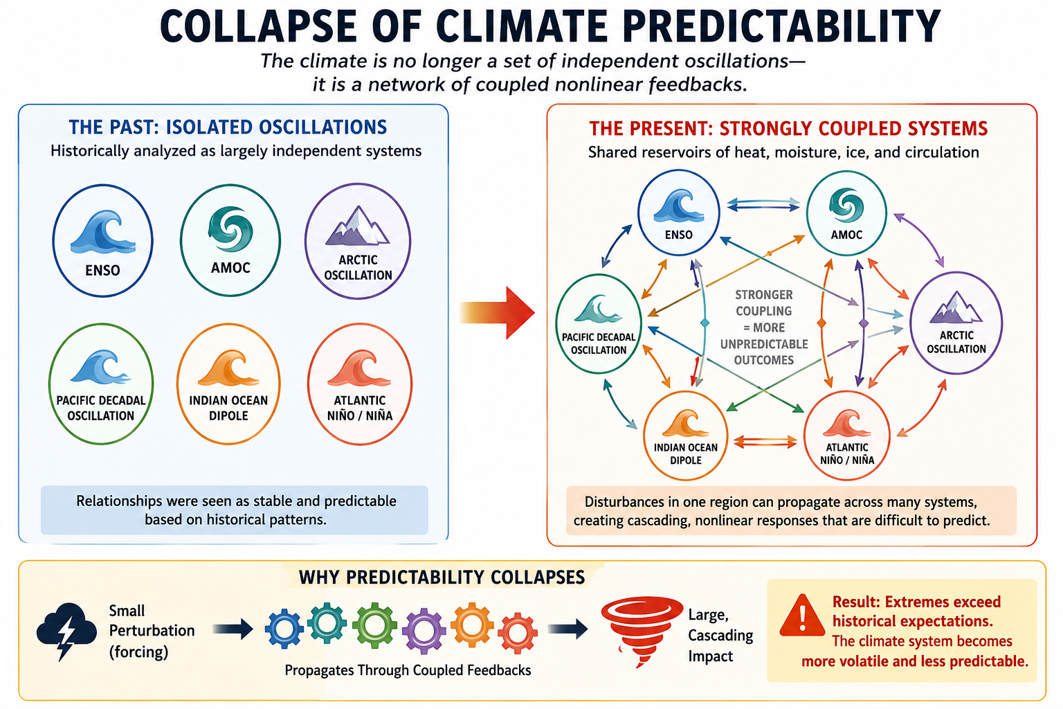
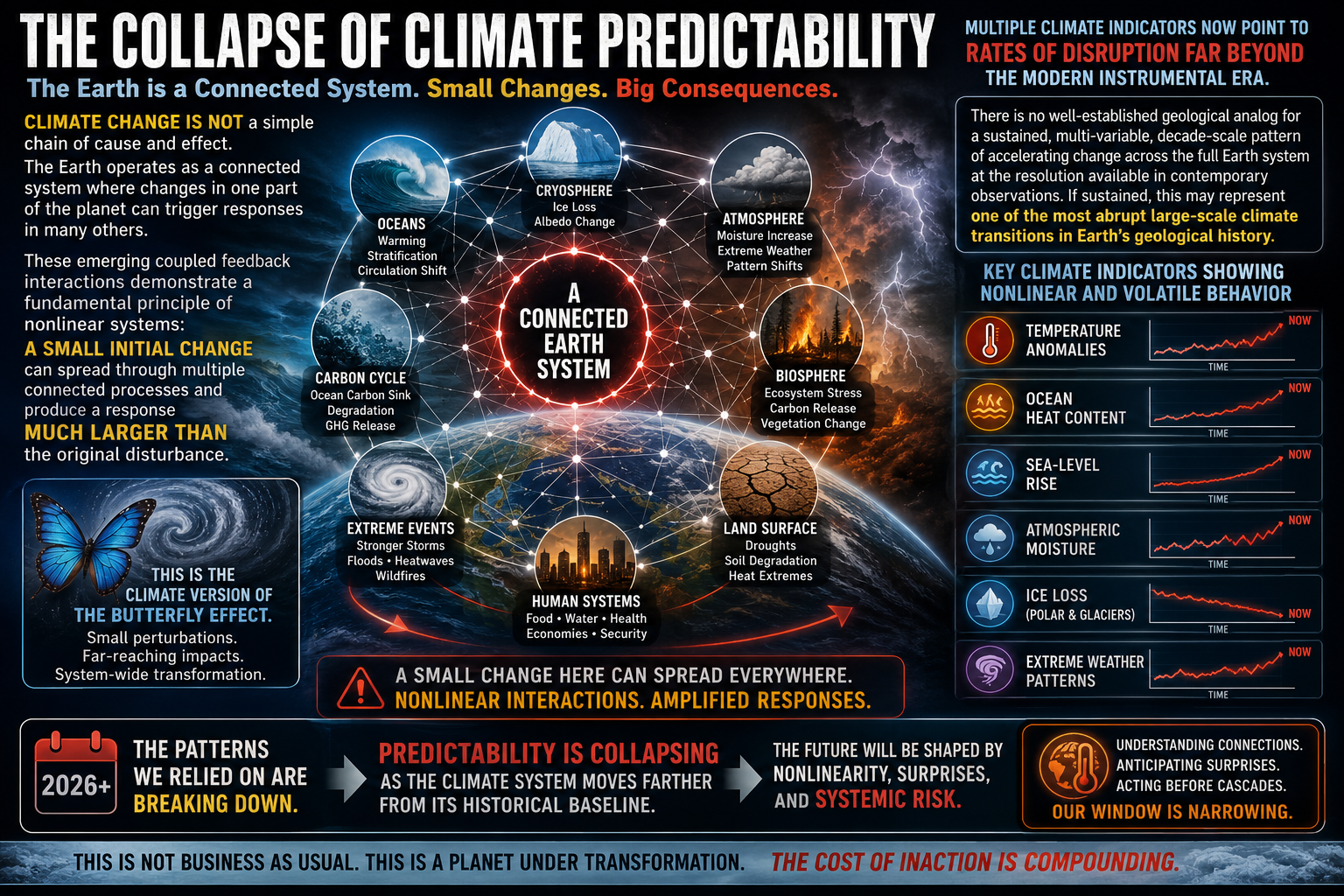
For much of the modern scientific era, Earth’s major climate oscillations were studied as largely independent systems. Phenomena such as the El Niño–Southern Oscillation (ENSO), the Atlantic Meridional Overturning Circulation (AMOC), the Arctic Oscillation (AO), the Pacific Decadal Oscillation (PDO), the Indian Ocean Dipole (IOD), and the Atlantic Niño/Niña each possessed recognizable patterns, historical relationships, and reasonably predictable behavior.
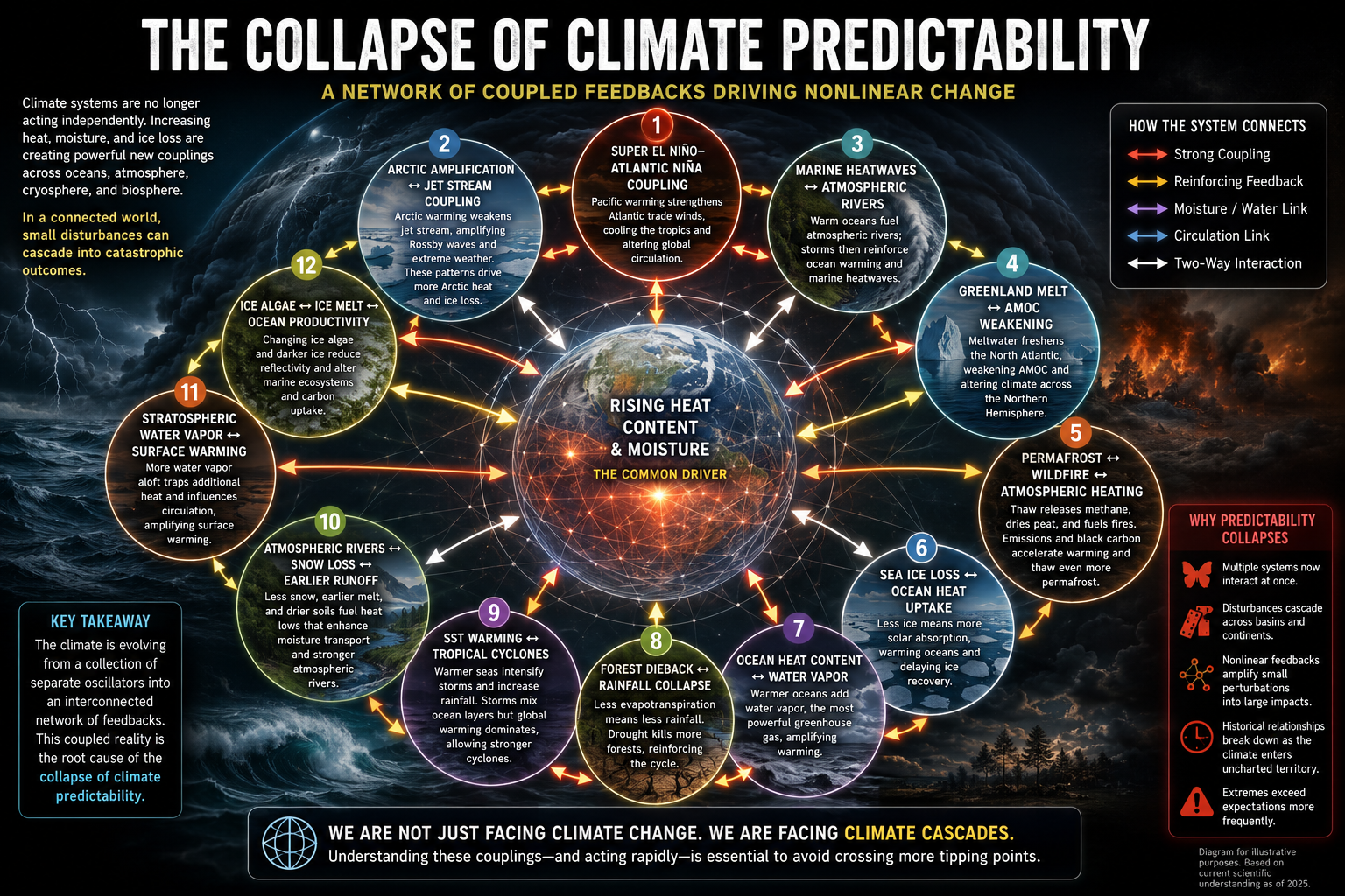
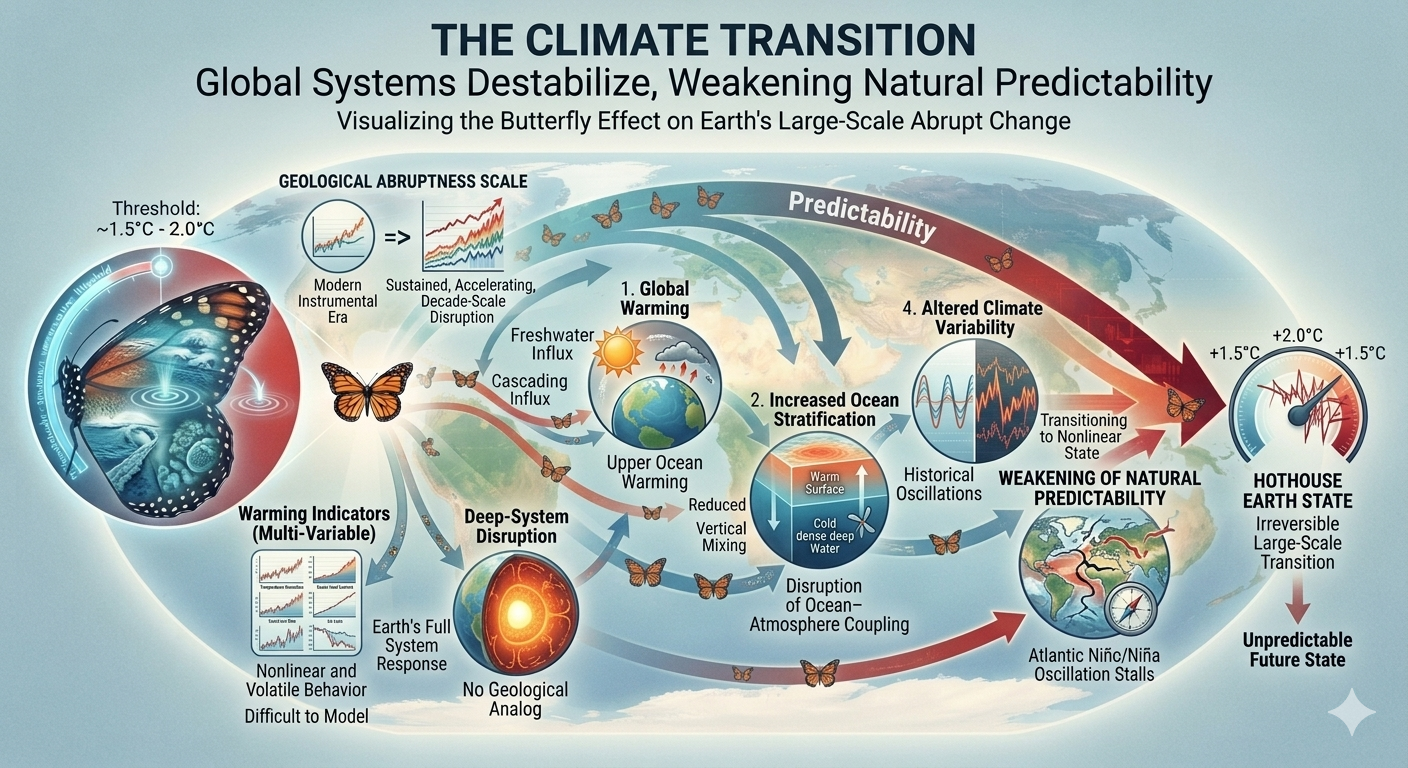
Today, however, a growing body of observations suggests these systems are becoming increasingly interconnected through shared reservoirs of heat, moisture, ice, and atmospheric circulation. Rather than behaving as isolated oscillators, they are evolving into a tightly coupled network in which disturbances propagate across multiple components of the Earth system. This increasing connectivity reduces the reliability of historical climate relationships and contributes to what can be described as the collapse of climate predictability.
From Independent Oscillators to a Coupled System
Classical climatology often treated Earth’s major modes of variability as separate oscillations whose interactions were relatively weak and occurred over well-defined time scales.
These oscillations remain useful conceptual tools, but they no longer appear to behave as isolated components. Instead, they increasingly exchange energy through atmospheric circulation, ocean heat transport, cryospheric change, and hydrologic feedbacks.
The climate system is transitioning from a collection of loosely connected oscillators to a highly interconnected nonlinear network.
The Common Driver: Earth’s Growing Energy Imbalance
The increasing coupling among climate systems is not random.
It is driven by a steadily increasing accumulation of heat within the Earth system.
More than 90 percent of the excess energy trapped by greenhouse gases is absorbed by the oceans. Rising ocean heat content increases evaporation, atmospheric water vapor, sea surface temperatures, and latent heat available to storms. At the same time, declining sea ice reduces Earth’s reflectivity, allowing additional solar energy to be absorbed. Melting glaciers introduce freshwater into the oceans, altering circulation patterns, while warming soils and thawing permafrost release additional greenhouse gases.
These processes all originate from the same growing energy imbalance, linking climate systems that historically behaved more independently.
Emerging Climate Couplings
Numerous examples illustrate this increasing interconnectedness.
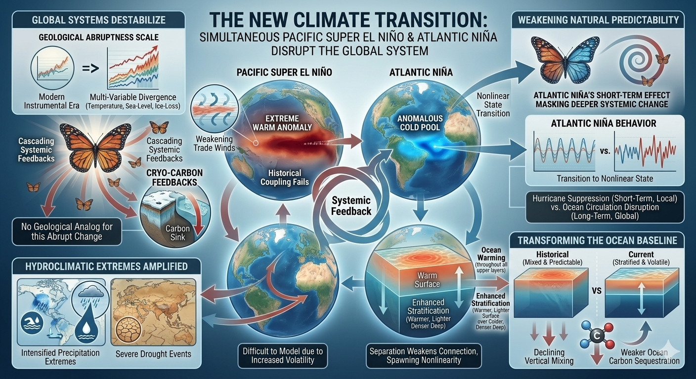
Super El Niño–Atlantic Niña
Exceptional Pacific warming modifies atmospheric circulation, strengthening Atlantic trade winds and promoting cooling in portions of the tropical Atlantic. The altered Atlantic circulation then feeds back into global atmospheric patterns, influencing hurricane development, African rainfall, and Amazon precipitation.
Arctic Amplification–Jet Stream Coupling
Rapid Arctic warming weakens the north-south temperature gradient that maintains the polar jet stream. The resulting slower, more meandering jet stream favors persistent blocking patterns, prolonged heat domes, stalled storms, and extended droughts. Those weather extremes further accelerate Arctic warming through enhanced ice loss and wildfire activity.
Greenland Melt–AMOC Coupling
Accelerated melting of the Greenland Ice Sheet introduces freshwater into the North Atlantic, reducing salinity and slowing deep-water formation. A weaker AMOC alters weather patterns across the Northern Hemisphere, changing precipitation and temperature patterns that can further influence Greenland’s mass balance.
Marine Heatwaves–Atmospheric Rivers
Warmer oceans increase evaporation and atmospheric moisture. Enhanced water vapor intensifies atmospheric rivers, producing heavier precipitation while simultaneously reinforcing marine heatwaves through changes in ocean mixing and heat distribution.
Permafrost–Wildfire–Atmosphere Coupling
Permafrost thaw releases methane and dries peatlands, increasing wildfire activity. Wildfires emit greenhouse gases and black carbon, which darkens snow and ice surfaces, accelerating melting and further warming high-latitude regions.
Forest Dieback–Rainfall Coupling
Forests recycle enormous quantities of moisture through evapotranspiration. As forests decline from heat, drought, or wildfire, atmospheric moisture recycling weakens, reducing rainfall and increasing drought severity, which in turn accelerates additional forest loss.
Why Predictability Is Declining
Historically, climate forecasting relied heavily on recurring relationships.
Meteorologists and climatologists could often estimate future conditions because the underlying oscillations behaved within relatively stable statistical boundaries.
As coupling strengthens, those assumptions become increasingly unreliable.
A disturbance originating in one ocean basin can now propagate through atmospheric circulation into multiple ocean basins, alter sea surface temperatures elsewhere, modify jet stream behavior, influence storm tracks, and feed back into the original disturbance.
Small changes no longer remain local.
Instead, they cascade through interconnected systems.
The result is increasing uncertainty, even while the underlying driver—Earth’s growing energy imbalance—continues to strengthen.
A Network of Nonlinear Feedbacks
This transition is fundamentally a problem of nonlinear dynamics.
In linear systems:
responses are generally proportional to the forcing;
small perturbations can produce disproportionately large responses;
interactions among multiple feedback loops amplify disturbances; and
outcomes become increasingly sensitive to initial conditions.
As climate systems become more strongly coupled, Earth’s behavior increasingly resembles a nonlinear network rather than a collection of independent oscillators.
This is the climate-scale manifestation of the Butterfly Effect.
Cascading Climate Responses
Once coupling strengthens sufficiently, climate events begin propagating across multiple systems.
Each step reinforces subsequent processes, creating cascading responses that are considerably larger than the original perturbation.
Beyond Traditional Climate Variability
Many recent extreme events have exceeded expectations based on historical climate statistics.
Persistent heat domes, multi-day atmospheric rivers, marine heatwaves, rapid intensification of tropical cyclones, widespread wildfire outbreaks, and simultaneous extremes occurring across multiple continents increasingly reflect the behavior of an interconnected system rather than isolated weather anomalies.
The climate is no longer responding solely through individual oscillations.
It is responding through interactions among oscillations.
A New Framework for Climate Science
Understanding future climate risk increasingly requires moving beyond analyses that focus on individual climate modes in isolation.
Future prediction will depend on understanding:
cross-basin ocean interactions;
atmospheric teleconnections;
cryosphere–ocean coupling;
biosphere–atmosphere feedbacks;
hydrologic amplification; and
nonlinear propagation through coupled climate networks.
The central scientific challenge is no longer identifying individual feedbacks, but understanding how those feedbacks interact simultaneously.
Conclusion
The growing accumulation of heat within Earth’s climate system is strengthening connections among atmospheric, oceanic, cryospheric, and biological processes. These interactions are transforming once largely independent climate oscillations into a coupled network of nonlinear feedbacks.
As coupling intensifies, disturbances spread more efficiently across the Earth system, historical relationships become less reliable, and extreme events increasingly exceed expectations derived from the past. The resulting decline in predictability is not evidence that the climate has become random. Rather, it reflects the behavior of a highly interconnected nonlinear system whose responses are increasingly governed by cascading interactions instead of isolated processes.
The collapse of climate predictability is therefore best understood not as the failure of climate science, but as the emergence of a new climatic regime—one in which understanding the connections between Earth’s major systems becomes as important as understanding the systems themselves.
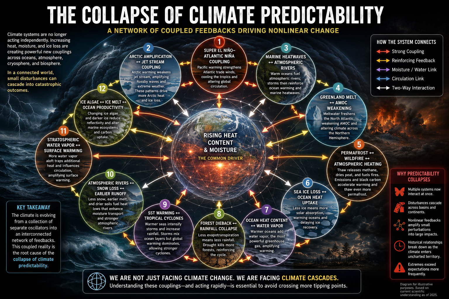
The Super El Niño–Atlantic Niña coupling is one of the clearest examples of how formerly semi-independent climate oscillations are becoming more tightly linked in a warmer world. But it is far from the only coupling now being observed. Increasing ocean heat content, declining sea ice, changing atmospheric circulation, and enhanced moisture transport are creating new interactions that reduce the reliability of historical climate relationships.
Here’s a framework of the most important coupled systems contributing to the collapse of climate predictability.
1. Super El Niño ↔ Atlantic Niña
(Cross-basin ocean-atmosphere coupling)
Mechanism
Exceptional warming in the equatorial Pacific alters the Walker Circulation.
Stronger trades cool the eastern tropical Atlantic.
The Atlantic then feeds back into global circulation.
Consequences
Hurricane seasons become less predictable.
African monsoon shifts.
Amazon rainfall changes.
Jet streams reorganize globally.
This is no longer simply ENSO affecting the Atlantic—it becomes a two-way coupled system.
2. Arctic Amplification ↔ Jet Stream Coupling
6
As the Arctic warms 3–4 times faster than the global average:
temperature gradients weaken
jet stream slows
Rossby waves amplify
blocking patterns persist longer
The weakened jet stream then:
allows additional Arctic heat transport
increases sea ice melt
reinforces Arctic amplification
This positive feedback produces
prolonged heat domes
stalled atmospheric rivers
persistent droughts
multi-day flooding events
3. Marine Heatwaves ↔ Atmospheric Rivers
Warm oceans increase
evaporation
atmospheric water vapor
latent heat release
That additional moisture intensifies atmospheric rivers.
The storms themselves:
warm coastal oceans
reduce ocean mixing
reinforce marine heatwaves
Result:
stronger flooding
stronger coastal storms
longer marine heatwaves
4. Greenland Melt ↔ AMOC Weakening
5
Greenland melt adds enormous volumes of freshwater.
Freshwater reduces salinity.
Lower salinity reduces deep water formation.
The Atlantic Meridional Overturning Circulation (AMOC) weakens.
A weaker AMOC then alters
North Atlantic temperatures
European weather
tropical rainfall
hurricane development
Those changes affect Greenland snowfall and melting, completing another coupled feedback.
5. Permafrost ↔ Wildfire ↔ Atmospheric Heating
One of the fastest emerging feedbacks.
Warming causes:
permafrost thaw
methane release
peat drying
Dry peat fuels zombie fires.
Wildfires release
CO₂
methane
black carbon
Black carbon settles on Arctic snow.
Lower albedo accelerates melting.
Additional warming thaws even more permafrost.
6. Sea Ice Loss ↔ Ocean Heat Uptake
Sea ice reflects sunlight.
Open ocean absorbs sunlight.
As sea ice retreats:
solar absorption increases dramatically
upper ocean warms
autumn freeze is delayed
winter ice becomes thinner
The thinner ice melts faster the following year.
This coupling is one reason Arctic warming has accelerated so rapidly.
7. Ocean Heat Content ↔ Water Vapor
This is perhaps the most fundamental coupling.
Warmer oceans
↓
greater evaporation
↓
more atmospheric water vapor
↓
stronger greenhouse effect
↓
warmer oceans
Water vapor also fuels:
heavier rainfall
stronger hurricanes
more latent heat release
explosive convection
8. Forest Dieback ↔ Rainfall Collapse
5
Forests recycle enormous amounts of moisture.
Loss of forests means
less evapotranspiration
less rainfall
longer droughts
Drought kills more forests.
This coupling is becoming increasingly important in
Amazon
Boreal Canada
Siberia
9. Sea Surface Temperature ↔ Tropical Cyclones
Warmer oceans produce
stronger hurricanes
slower-moving hurricanes
greater rainfall
Storms mix the upper ocean.
Sometimes mixing cools local waters.
But globally, warming oceans increasingly outweigh this cooling, allowing storms to intensify more rapidly and maintain higher rainfall rates.
10. Atmospheric Rivers ↔ Snow Loss ↔ Earlier Runoff
Reduced mountain snowpack means
less spring melt
drier soils
warmer land surfaces
Warmer land strengthens heat lows.
Heat lows enhance moisture transport.
Atmospheric rivers become stronger.
11. Stratospheric Water Vapor ↔ Surface Warming
Increasing methane oxidation and occasional injections of water vapor into the stratosphere increase its greenhouse effect.
Additional warming raises sea surface temperatures, which increase evaporation and atmospheric moisture, further reinforcing warming.
12. Ice Algae ↔ Ice Melt ↔ Ocean Productivity
Melting sea ice changes the timing and distribution of ice algae blooms.
Dark algal communities can reduce ice reflectivity locally, while shifts in marine ecosystems affect carbon uptake. Although smaller than many other feedbacks, these biological changes interact with physical ice loss and ocean warming.
Why This Leads to the Collapse of Climate Predictability
Historically, climate scientists often analyzed these systems as largely independent oscillations:
ENSO
AMOC
Arctic Oscillation
Pacific Decadal Oscillation
Indian Ocean Dipole
Atlantic Niño/Niña
Increasing evidence shows they are interacting more strongly through shared reservoirs of heat, moisture, ice, and atmospheric circulation. As coupling strengthens, disturbances in one region can propagate across multiple climate systems, creating cascading responses that are difficult to anticipate with historical relationships alone.
Instead of isolated oscillators, the climate increasingly behaves as a network of coupled nonlinear feedbacks. In such systems, modest perturbations can cascade through multiple connected processes, producing responses much larger than the initial forcing. This interconnected behavior helps explain why recent extremes have often exceeded expectations based on past climate variability and why forecasting becomes more challenging as the system evolves.
Multiple climate indicators now point to rates of warming-related disruption far beyond those observed during the modern instrumental era. There is no well-established geological analog for a sustained, multi-variable, decade-scale pattern of accelerating change across the full Earth system at the resolution available in contemporary observations. If sustained, this may represent one of the most abrupt large-scale climate transitions in Earth’s geological history.
Many of the climate indicators traditionally used for forecasting are exhibiting increasingly nonlinear and volatile behavior. Temperature anomalies, ocean heat content, sea-level rise, atmospheric moisture, ice loss, and extreme weather patterns are showing changes that are becoming more difficult to model using assumptions based primarily on historical variability.
Abstract
The simultaneous occurrence of an extreme Pacific Super El Niño and an anomalous Atlantic Niña represents a significant disruption of historically observed ocean–atmosphere interactions. These coupled climate anomalies illustrate how anthropogenic warming is altering the baseline state of Earth’s climate system, reducing predictability, amplifying hydroclimatic extremes, and accelerating interconnected feedback mechanisms. While an Atlantic Niña pattern may temporarily suppress Atlantic hurricane activity through increased atmospheric stability and wind shear, this short-term effect masks deeper systemic changes occurring within global ocean circulation, carbon cycling, and energy redistribution.
Climate change is increasingly modifying the physical conditions under which natural climate oscillations such as El Niño–Southern Oscillation (ENSO) and Atlantic Niño variability operate. Warmer ocean surfaces, enhanced stratification, declining vertical mixing, and changing circulation patterns are transforming previously stable climate relationships into increasingly nonlinear and difficult-to-predict interactions. These changes threaten to intensify global precipitation extremes, weaken ocean carbon sequestration, and accelerate reinforcing feedback loops involving greenhouse gas emissions, ocean warming, and cryosphere loss.
1. Introduction: A Changing Climate Baseline
Earth’s climate system is governed by complex interactions between the atmosphere, oceans, cryosphere, and biosphere. Natural climate oscillations, including Pacific El Niño events and Atlantic Niño/Niña variability, have historically provided a degree of predictability by influencing global temperature patterns, rainfall distributions, and storm activity.
However, climate change is altering the fundamental conditions under which these oscillations occur. The emergence of an extreme Pacific Super El Niño coinciding with an Atlantic Niña demonstrates a growing departure from historical climate behavior. Rather than acting as isolated events, these anomalies increasingly interact within a warmer planetary system, producing nonlinear responses that amplify regional and global impacts.
The key concern is not the individual climate pattern itself, but the changing background state in which these patterns develop.
2. Weakening of Natural Climate Predictability
2.1 Disruption of Ocean–Atmosphere Coupling
The Atlantic Niño/Niña cycle depends on interactions between surface ocean temperatures, subsurface heat content, atmospheric circulation, and equatorial wind patterns. Under historical conditions, these interactions produced recognizable oscillations that contributed to seasonal climate predictability.
Global warming is now modifying this relationship.
As greenhouse gas accumulation increases ocean heat content, warming is occurring throughout the upper ocean layers. This enhanced surface warming increases ocean stratification—the separation between warmer, lighter surface water and colder, denser deep water.
The result is a reduction in vertical ocean mixing:Ocean Warming→Increased Stratification→Reduced Vertical Mixing→Altered Climate Variability
This separation weakens the connection between surface conditions and deeper ocean processes, making climate oscillations more irregular and reducing the reliability of historical forecasting models.
The Atlantic Niño/Niña system is therefore transitioning from a relatively predictable oscillatory behavior toward a more complex, nonlinear state influenced by persistent anthropogenic forcing.
3. Global Redistribution of Rainfall Extremes
The interaction between a Pacific Super El Niño and Atlantic Niña creates a highly disrupted global precipitation pattern.
3.1 Extreme Flooding in West Africa
An intensified Atlantic Niña can strengthen atmospheric circulation patterns associated with the West African monsoon.
Enhanced ocean–atmosphere energy exchange increases moisture transport into the Gulf of Guinea region, potentially producing:
Extreme rainfall events
River flooding
Agricultural disruption
Infrastructure damage
Increased risks to vulnerable populations
Rather than representing a simple regional anomaly, these changes demonstrate how altered ocean temperatures can reorganize atmospheric circulation thousands of kilometers away.
3.2 Intensified Drought in Northeastern South America
At the same time, Atlantic Niña conditions can reduce moisture transport into northeastern South America.
When combined with Pacific El Niño influences, this can amplify drought conditions through:
Reduced atmospheric moisture availability
Persistent high-pressure systems
Increased evaporation from warming land surfaces
Reduced soil moisture retention
The result is a climate paradox: one region experiences catastrophic flooding while another experiences severe drought, both driven by the same reorganizing global climate system.
4. Amplification of Climate Feedback Loops
The 2026 ocean–atmosphere configuration illustrates how climate variability can interact with long-term warming trends to activate reinforcing feedback mechanisms.
A simplified representation is:Ocean Warming→Stronger Stratification→Reduced Mixing↓Increased Greenhouse Gas Release→Accelerated Warming→Further Ocean Warming
These feedbacks transform climate change from a linear response into a nonlinear system where small perturbations can trigger increasingly larger consequences.
5. The Marine Methane Feedback Loop
5.1 Stratification and Ocean Biological Disruption
The ocean plays a critical role in regulating atmospheric greenhouse gases. However, warming-driven stratification threatens this regulatory function.
Normally, ocean circulation transports nutrients such as phosphate and nitrogen from deep waters toward the surface, supporting marine ecosystems and biological carbon uptake.
As stratification increases:Surface Warming→Reduced Nutrient Mixing→Altered Marine Ecosystems
Nutrient limitation changes microbial communities and can increase conditions favorable for methane-producing organisms.
5.2 Methane Amplification
Methane (CH4) is a highly effective greenhouse gas, particularly over shorter atmospheric timescales.
Over a 20-year period, methane has a substantially greater warming influence than carbon dioxide (CO2).
This represents a positive feedback loop in which warming creates conditions that generate additional warming.
6. Degradation of the Ocean Carbon Sink
6.1 The Ocean as a Global Carbon Reservoir
The ocean currently absorbs approximately one-quarter of anthropogenic carbon dioxide emissions, functioning as one of Earth’s most important climate stabilizing mechanisms.
This process depends heavily on ocean circulation systems, including the Atlantic Meridional Overturning Circulation (AMOC).
The AMOC transports warm surface water northward, where cooling increases density and allows carbon-rich water to sink into the deep ocean.
6.2 Weakening Carbon Removal Capacity
Climate change threatens this process through:
Rising ocean temperatures
Increased freshwater input from melting ice sheets
Reduced deep-water formation
Increased ocean stratification
Warmer water absorbs less dissolved gas, while weaker circulation reduces the transport of carbon into the deep ocean.
The resulting feedback is:Ocean Warming→Reduced Carbon Storage→More Atmospheric CO2→Further Warming
A weakened ocean carbon sink represents a fundamental shift from a stabilizing Earth system component toward a potential climate amplifier.
7. The Ice–Albedo Feedback Loop
Super El Niño events often produce temporary increases in global temperatures by redistributing stored ocean heat into the atmosphere.
During these periods, extreme heat accelerates melting of:
Arctic sea ice
Mountain glaciers
Polar ice sheets
The loss of reflective ice surfaces activates the ice–albedo feedback:Ice Loss→Reduced Solar Reflection→Increased Ocean Heat Absorption→Accelerated Ice Loss
Bright ice reflects incoming solar radiation back into space. Dark ocean water absorbs much more solar energy, increasing local warming and accelerating further melting.
This creates a self-reinforcing cycle affecting polar regions and global temperature patterns.
8. Conclusion: From Climate Variability to Climate System Transformation
The interaction between a Pacific Super El Niño and an Atlantic Niña provides a window into a rapidly changing climate system. While individual climate anomalies may temporarily produce localized benefits, such as reduced Atlantic hurricane activity, these short-term effects do not indicate increased climate stability.
Instead, the emergence of unusual ocean–atmosphere configurations reflects deeper structural changes:
Reduced predictability of natural climate oscillations
Increasing precipitation extremes
Weakening ocean carbon storage
Intensifying greenhouse gas feedback loops
Accelerating cryosphere loss
Climate change is not simply increasing average global temperatures; it is reorganizing the interactions between Earth’s major systems. The greatest risk arises from the increasing coupling of multiple feedback processes, where changes in one component of the climate system amplify changes elsewhere.
The future trajectory of climate stability will depend not only on reducing greenhouse gas emissions but also on understanding and monitoring these increasingly interconnected nonlinear responses within the Earth system.
Introduction: The Hidden Connections Driving Climate Change
Climate change is not a simple chain of cause and effect. The Earth operates as a connected system where changes in one part of the planet can trigger responses in many others. These emerging coupled feedback interactions demonstrate a fundamental principle of nonlinear systems: a small initial change can spread through multiple connected processes and produce a response much larger than the original disturbance. This is the climate version of the Butterfly Effect.
Climate feedbacks do not operate independently. Instead, they interact as a vast network linking the atmosphere, oceans, ice sheets, forests, soils, and ecosystems. When one feedback strengthens another, the combined effect can become greater than the sum of the individual parts. This is why climate change can sometimes accelerate faster than expected and why predicting future changes is so challenging.
From Individual Feedbacks to Climate Cascades
A traditional climate feedback is often described as a single process:
warming melts ice,
melting ice reduces reflectivity,
reduced reflectivity causes more warming.
However, the real climate system is more complex. One feedback can activate several others, creating a chain reaction across different parts of the planet.
These connected processes are called coupled feedback interactions. They occur when multiple feedbacks reinforce one another, creating cascading effects that cannot be understood by studying each process separately.
Wildfires: From Local Fires to Global Feedbacks
A powerful example begins with heat and drought.
As temperatures rise and soils dry, forests become more vulnerable to large wildfires. These fires release carbon dioxide stored in trees and soils, adding more greenhouse gases to the atmosphere. They also produce black carbon, or soot, which can travel long distances and settle on snow, glaciers, and Arctic sea ice.
Darkened ice and snow absorb more sunlight than clean, reflective surfaces. This increases melting, exposes darker land and ocean surfaces, and allows even more solar energy to be absorbed.
At the same time, burned forests lose their ability to remove carbon dioxide from the atmosphere. A regional drought can therefore trigger a chain of connected responses involving the atmosphere, forests, ice, and oceans.
A single wildfire can become part of a much larger climate feedback network.
Arctic Permafrost: The Sleeping Carbon Reservoir
The Arctic contains enormous amounts of carbon stored in frozen soils known as permafrost. As the Arctic warms, this frozen ground begins to thaw.
When permafrost melts:
microorganisms break down ancient organic material,
carbon dioxide and methane are released,
additional greenhouse gases enter the atmosphere,
warming increases further.
Thawing permafrost can also create thermokarst lakes—collapsed areas filled with water. These lakes absorb heat more efficiently than frozen ground, accelerating nearby thaw.
Another unusual example is the rise of zombie fires. These underground fires can continue burning beneath snow throughout the winter, then reappear during warmer seasons. They release carbon, damage vegetation, and accelerate the loss of the insulating layers that protect permafrost.
Together, permafrost thaw, methane release, thermokarst lakes, and zombie fires form a connected Arctic amplification system.
Greenland Ice Algae: When Life Darkens Ice
Greenland provides one of the most surprising examples of a biological climate feedback.
As temperatures rise, more snow and ice melt during summer. This exposes surfaces where microscopic algae can grow. These algae contain dark pigments that reduce the brightness of the ice.
Normally, bright ice reflects sunlight back into space. Darker ice absorbs more solar energy.
The result:
melting ice → more algae growth → darker ice → more solar absorption → faster melting
As melting increases, more liquid water becomes available, creating conditions that can support additional algal growth. A biological process becomes directly connected to the physical loss of an ice sheet.
Oceans and the Atmosphere: A Heat and Moisture Engine
The oceans absorb most of the excess heat trapped by greenhouse gases. As ocean temperatures rise, evaporation increases, adding more water vapor to the atmosphere.
Water vapor is itself a greenhouse gas, creating additional warming.
A warmer ocean and atmosphere can contribute to:
stronger atmospheric rivers,
heavier rainfall events,
more intense tropical storms,
longer-lasting marine heatwaves.
At the same time, warmer oceans can become less effective at absorbing carbon dioxide. Marine heatwaves can also damage ecosystems such as kelp forests and phytoplankton communities that help remove carbon from the atmosphere.
The ocean, atmosphere, and biosphere therefore form a tightly connected climate system.
Vegetation Changes: The Arctic Landscape Transforms
Climate change can also reshape ecosystems in ways that amplify warming.
As Arctic temperatures increase, shrubs expand into areas that were previously dominated by low vegetation. These darker shrubs absorb more sunlight than snow-covered tundra.
Shrubs also trap more snow during winter. Deeper snow acts like a blanket, keeping the ground warmer and accelerating permafrost thaw.
A similar process occurs in forests. Warmer winters allow pests such as bark beetles to survive in greater numbers. Large areas of weakened forest can then become vulnerable to wildfire, releasing more carbon and reducing future carbon storage.
The Bigger Picture: Earth as a Connected System
These examples reveal an important shift in how we understand climate change.
The Earth system is not simply a collection of separate feedback loops. It is a network of interacting systems where changes in one area can activate responses elsewhere.
A warming ocean can influence the atmosphere. A wildfire can influence ice melt. Melting ice can influence ecosystems. Changing ecosystems can influence greenhouse gases.
These connections create climate cascades—chains of interacting processes that can amplify change throughout the planet.
The future of climate change will depend not only on the amount of greenhouse gases added to the atmosphere, but also on how these interconnected feedbacks evolve, interact, and influence one another.
Understanding these hidden connections is essential for understanding why climate change is not just warming—it is a rapidly evolving Earth system response.