Nighttime minimum temperatures are increasing in many regions at a faster rate than daytime maximum temperatures, representing a critical but underappreciated dimension of climate change. Because human and ecosystem recovery from heat stress depends heavily on nocturnal cooling, this trend has important implications for health outcomes, agriculture, energy demand, and ecological stability. This paper examines the role of warming nights in transforming extreme heat from a diurnal hazard into a sustained 24-hour physiological stress regime.
1. Introduction
Extreme heat is typically characterized using daytime maximum temperatures. However, increasing evidence indicates that nighttime minimum temperatures are rising more rapidly than daytime maxima in many regions. This shift is particularly significant because nighttime cooling is a primary mechanism through which biological systems recover from daytime thermal stress.
The loss of adequate nighttime relief effectively transforms heat waves from short-duration exposure events into sustained multi-day stress periods.
2. Observed Trend in Nighttime Minimum Temperatures
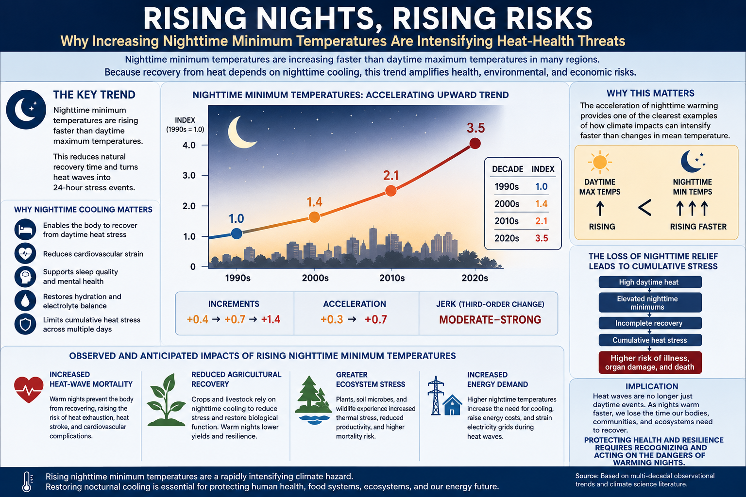
Nighttime warming has accelerated across multiple observational datasets. A simplified index representation illustrates the nonlinear increase in nighttime minimum temperature impacts:
Decade
Index
1990s (baseline)
1.0
2000s
1.4
2010s
2.1
2020s
3.5
Incremental change:
1990s → 2000s: +0.4
2000s → 2010s: +0.7
2010s → 2020s: +1.4
Acceleration:
First difference: +0.3 → +0.7
Second difference: increasing magnitude of change
Qualitative classification:
Jerk (third-order change): Moderate to Strong
This structure indicates not only rising nighttime temperatures, but also an acceleration in the rate at which those increases are occurring.
3. Physical Mechanisms
Several interacting mechanisms contribute to enhanced nighttime warming:
Increased atmospheric greenhouse gas concentrations reducing outgoing longwave radiation
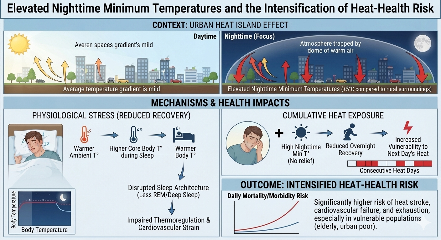
Urban heat island effects due to thermal storage in built environments
Reduced cloud radiative cooling efficiency in some regions
Heat retention in oceans and adjacent land systems
Together, these processes suppress nighttime energy loss and elevate minimum temperatures.
4. Physiological Significance of Nighttime Cooling
Biological recovery from heat stress depends strongly on nighttime temperature reduction. When nighttime minima remain elevated:
Core body temperature recovery is incomplete
Cardiovascular strain persists overnight
Sleep quality is degraded
Hydration and electrolyte balance are not restored
Cumulative heat stress increases across consecutive days
As a result, heat waves become continuous physiological stress events rather than discrete daytime exposures.
5. Observed Impacts of Rising Nighttime Temperatures
The acceleration of nighttime warming is associated with multiple observed and projected impacts:
Increased heat-wave mortality
Reduced agricultural recovery and crop resilience
Greater ecosystem stress and reduced plant productivity
Increased residential and grid energy demand for nighttime cooling
These impacts highlight the systemic nature of nighttime temperature changes across human and natural systems.
6. Discussion
The increasing divergence between nighttime minimum and daytime maximum temperature trends suggests a structural shift in the nature of heat extremes. Rather than being driven solely by peak daytime conditions, modern heat risk is increasingly determined by the loss of nocturnal recovery capacity.
This shift implies that heat extremes should be conceptualized as integrated 24-hour thermal stress regimes rather than isolated daytime events.
7. Conclusion
Nighttime minimum temperatures represent a rapidly intensifying component of climate change with disproportionate impacts on human health, agriculture, ecosystems, and energy systems. The observed asymmetry—where nighttime lows are increasing faster than daytime highs in many regions—highlights the importance of diurnal temperature structure in climate risk assessment. As nocturnal cooling declines, heat waves increasingly function less as short-lived peaks and more as sustained, cumulative thermal stress events.
As temperatures rise, cooling demand increases sharply. This drives a cascading set of system stresses:
higher electricity demand during heat waves
strain on generation and transmission infrastructure
increased water demand in some regions for cooling and supply stability
and, in grids still reliant on fossil fuels, increased emissions during peak demand periods
This creates a reinforcing sequence:
more heat → more cooling demand → higher energy use → higher emissions → further warming → more heat
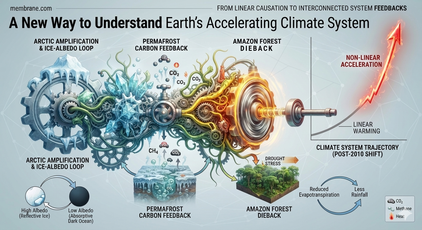
In practice, what emerges is not a single isolated feedback loop, but a coupled network of reinforcing systems—biophysical (permafrost thaw, forest stress and mortality, wildfire regimes, hydrological intensification) and socioeconomic (energy demand, infrastructure constraints, and grid response). These systems can interact nonlinearly, particularly under sustained warming and extreme heat conditions.
The key point is that these feedbacks are already operating, but their magnitude, interaction strength, and long-term dominance relative to human emissions vary by region, sector, and timeframe. Reducing risk ultimately depends on rapidly reducing greenhouse gas emissions, especially from fossil fuel combustion, while adapting infrastructure to rising heat extremes.
The U.S. labor force participation rate now stands at 61.5%, according to the latest Bureau of Labor Statistics (BLS) June 2026 report. This metric measures the share of the civilian population aged 16 and older that is either employed or actively seeking work, and it declined from 61.8% in the prior reading.
Within the broader non-participating population, only a small segment is considered even loosely attached to the labor market. Approximately 1.76 million people are classified as “marginally attached” to the labor force—individuals who want a job and have looked for work within the past 12 months, but have not searched in the past four weeks. Of these, about 477,000 are “discouraged workers,” meaning they believe no jobs are available for them or that they lack the skills required to obtain employment.
The latest BLS June 2026 employment report highlights a notable shift in labor force dynamics. Roughly 720,000 people left the labor force, contributing to the decline in the participation rate from 61.8% to 61.5%.
This decline helps explain the apparent contradiction in the headline employment figures. The economy added a modest 57,000 jobs, and the official unemployment rate edged down from 4.3% to 4.2%. However, this improvement is partly driven by a smaller labor force rather than a surge in hiring, as fewer people were actively seeking work during the reporting period.
Intergovernmental Panel on Climate Change (2021). Climate Change 2021: The Physical Science Basis. Cambridge University Press.
Intergovernmental Panel on Climate Change (2022). Climate Change 2022: Impacts, Adaptation and Vulnerability. Cambridge University Press.
World Meteorological Organization. (2024). State of the Global Climate 2024.
Feng, Z., De Marco, A., Anav, A., et al. (2022). Economic losses due to ozone impacts on global crop production. Global Change Biology.
Ainsworth, E. A.. (2017). Understanding and improving global crop response to ozone pollution. The Plant Journal, 90, 886–897.
Emberson, L. D., Ashmore, M. R., et al. (2000). Modelling stomatal ozone flux across Europe. Environmental Pollution, 109, 403–413.
Sitch, S., Cox, P. M., Collins, W. J., et al. (2007). Indirect radiative forcing of climate change through ozone effects on the land-carbon sink. Nature, 448, 791–794.
Lombardozzi, D., Levis, S., Bonan, G., et al. (2015). The influence of chronic ozone exposure on global carbon cycling. Journal of Climate.
Jiang, X., et al. (2026). Fires Reverse Progress Toward Ozone Air Quality Standards in the United States. Science.
United States Environmental Protection Agency. Integrated Science Assessment for Ozone and Related Photochemical Oxidants (latest edition).
United States Environmental Protection Agency. Health Effects of Ozone Pollution.
National Oceanic and Atmospheric Administration. Global Monitoring Laboratory—Greenhouse Gases and Atmospheric Composition.
National Aeronautics and Space Administration. Earth Observatory. Ground-Level Ozone.
Copernicus Atmosphere Monitoring Service. Annual reports on global atmospheric composition and wildfire emissions.
Global Carbon Project. (2024). Global Carbon Budget 2024.
Anderegg, W. R. L., et al. (2020). Climate-driven risks to the climate mitigation potential of forests. Science.
Pan, Y., et al. (2011). A large and persistent carbon sink in the world’s forests. Science, 333, 988–993.
Hubau, W., et al. (2020). Asynchronous carbon sink saturation in African and Amazonian tropical forests. Nature.
Brienen, R. J. W., et al. (2015). Long-term decline of the Amazon carbon sink. Nature.
Bastos, A., et al. (2023). Increasing climate extremes are weakening terrestrial carbon sinks. Nature Climate Change.
Mills, G., et al. (2018). Tropospheric ozone assessment report: Present-day ozone distribution and impacts on vegetation. Elementa: Science of the Anthropocene.
World Health Organization. (2021). WHO Global Air Quality Guidelines.
Burney, J. & Ramanathan, V.. (2014). Recent climate and air pollution impacts on Indian agriculture. Proceedings of the National Academy of Sciences.
Avnery, S., et al. (2011). Global crop yield reductions due to surface ozone exposure. Atmospheric Environment.
Additional References: New Systems-Level Theory (“Ozone Feedback Theory”)
Lenton, T. M., et al. (2008). Tipping elements in the Earth’s climate system.Proceedings of the National Academy of Sciences.
Steffen, W., et al. (2018). Trajectories of the Earth System in the Anthropocene.Proceedings of the National Academy of Sciences.
Ripple, W. J., et al. (2024). The 2024 State of the Climate Report: Entering Uncharted Territory.BioScience.
Rockström, J., et al. (2023). Safe and just Earth system boundaries.Nature.
“This looks complicated.” True—it is complicated, and that’s part of the problem. The climate system involves interacting feedbacks across the atmosphere, oceans, biosphere, and cryosphere, so it can’t really be reduced to a single mechanism or slogan without losing important detail.
That’s exactly why we created this version as a public-access summary (roughly 6th–10th grade level)—to make the core ideas more accessible without requiring technical background.
But at the simplest level, the takeaway is straightforward: burning fossil fuels is driving the problem, and reducing those emissions is the most direct way to limit further warming and related impacts.
by Daniel Brouse
Executive Summary
For decades, climate change has often been described as a slow, gradual process. Rising temperatures, melting ice, and increasing sea levels were expected to unfold steadily over many generations.
That picture is changing.
Evidence from multiple independent observations now suggests that many parts of Earth’s climate system are no longer changing at constant rates. Instead, the rates of change themselves are increasing.
This distinction is important.
Instead of asking:
“How fast is sea level rising?”
we should increasingly ask:
“Is sea level rise itself speeding up?”
The same question applies to ocean warming, atmospheric moisture, marine heatwaves, wildfire conditions, and many other parts of the climate system.
This paper introduces a framework for examining the climate system as a single interconnected network whose major components exchange energy and reinforce one another through feedback loops. Rather than viewing each indicator independently, the framework evaluates how the entire system evolves together.
From Linear Change to Accelerating Change
Many natural systems change gradually.
Imagine driving a car at a constant speed.
Now imagine continually pressing the accelerator.
The difference is not simply that the car is moving—it is that the speed itself is increasing.
Earth’s climate increasingly appears to behave in the second way.
For much of the industrial era, many climate indicators changed relatively slowly.
Today, numerous observations show that several major Earth system components are accelerating simultaneously.
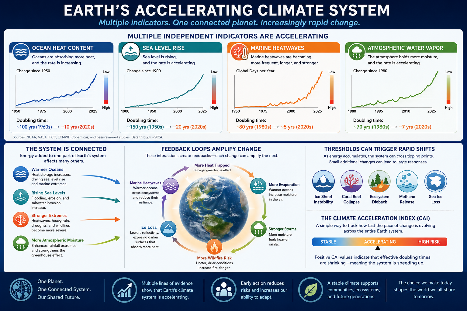
These include:
Ocean Heat Content
Global Sea Level
Marine Heatwaves
Atmospheric Water Vapor
Each represents a different part of Earth’s energy system, yet all respond to the same underlying planetary energy imbalance.
The Climate System Is Connected
Earth does not contain isolated climate systems.
Everything interacts.
As oceans absorb more heat:
seawater expands, raising sea levels
evaporation increases
atmospheric moisture rises
heavier rainfall becomes possible
marine heatwaves intensify
glaciers melt faster
ecosystems experience greater stress
These interactions create feedbacks.
A feedback occurs when one change amplifies another.
For example:
Ocean warming → More evaporation → More atmospheric water vapor → Stronger greenhouse trapping → Additional ocean warming
Each loop reinforces the next.
Instead of separate problems, these become parts of one larger system.
Why Doubling Times Matter
One useful way to understand acceleration is through doubling time.
Doubling time asks:
How long would it take for today’s value to double if the current rate continued?
If the doubling time becomes shorter, change is accelerating.
For example:
Doubling Time
Interpretation
100 years
Slow change
50 years
Changing faster
25 years
Acceleration increasing
10 years
Rapid acceleration
Shrinking doubling times indicate that the climate system is evolving more quickly than before.
They provide an intuitive way to compare very different climate indicators using a common measure.
Familiar Example
Many people are familiar with the power of compound interest. Historically, a diversified stock portfolio has returned about 10% per year over long periods (although actual returns vary from year to year).
At a 10% annual return, an investment doubles approximately every 7.2 years (using the Rule of 72).
FV=PV(1+r)n
Suppose you invest $10,000 at age 18 and leave it untouched until age 64—a period of 46 years.
Using annual compounding:FV=$10,000×(1.10)46 FV≈$803,731
That’s an increase by a factor of 80.4×.
Another way to see it is through doubling times:
Age 18: $10,000
Age 25 (1st doubling): $20,000
Age 32 (2nd): $40,000
Age 39 (3rd): $80,000
Age 46 (4th): $160,000
Age 53 (5th): $320,000
Age 60 (6th): $640,000
Age 64: About $804,000 (another four years of 10% growth beyond the sixth doubling)
This illustrates an important concept: the investment isn’t growing by the same dollar amount each year—it is growing by the same percentage. As the principal becomes larger, each year’s gain becomes dramatically larger than the previous year’s.
The compound interest example demonstrates why shrinking doubling times are so powerful. At a steady 10% annual return, an investment doubles about every seven years, allowing $10,000 to grow into more than $800,000 over a lifetime through the relentless mathematics of exponential growth. Climate change, however, may be even more concerning because the Earth’s effective doubling times are not remaining constant—they appear to be shrinking. In financial terms, it would be as if your investment initially doubled every 10 years, then every 5 years, then every 2 years, and eventually almost instantaneously. Each shortening of the doubling time means the system is accelerating, producing increasingly larger changes over increasingly shorter periods. As climate feedbacks strengthen, the accumulation and redistribution of energy through the oceans, atmosphere, ice sheets, and ecosystems can occur at an ever-faster pace. Just as investors celebrate faster compounding because it rapidly multiplies wealth, accelerating climate doubling times mean that warming, sea-level rise, extreme weather, and ecosystem disruption can compound much more quickly than linear thinking would suggest. The critical insight is not simply that the climate is changing, but that the pace of change itself is accelerating. In the limit, as the doubling time approaches zero, the system transitions toward an instantaneous-growth regime, where the characteristic timescale of change collapses and the climate system can respond far more rapidly than historical experience would suggest.
This is analogous to accelerating climate change. The Earth’s energy imbalance acts like the “interest rate.” If climate feedbacks strengthen over time, the effective growth rate increases and the doubling time shrinks. Just as a shortening doubling time makes an investment grow much faster, shrinking climate-system doubling times mean that changes in ocean heat, sea level, atmospheric moisture, and extreme events can accelerate much more rapidly than they did in previous decades.
A Shift Toward Threshold-Driven Dynamics
Many natural systems contain thresholds.
A bridge can withstand increasing weight until one additional truck causes failure.
A forest may tolerate drought for years before widespread wildfire suddenly erupts.
Ice sheets may melt slowly until structural weakening causes much faster ice loss.
Climate systems often behave similarly.
Energy accumulates gradually until internal stability begins to weaken.
Once thresholds are approached, relatively small additional warming can produce disproportionately large responses.
Scientists call this nonlinear behavior.
Instead of smooth change, the system begins responding through rapid jumps, stronger feedbacks, and cascading interactions.
Introducing the Climate Acceleration Index
To better understand this behavior, we introduce a simple concept called the Climate Acceleration Index (CAI).
Rather than measuring how large a climate variable becomes, the CAI measures how rapidly the pace of change itself is evolving.
Positive values indicate that effective doubling times are shrinking.
In plain language:
the system is speeding up
climate responses are occurring over shorter time scales
feedbacks are becoming increasingly important
The Climate Acceleration Index is intended as a system-wide diagnostic rather than a forecast.
Viewing the Entire Earth System
Traditional climate graphs usually display one variable at a time:
global temperature
sea level
ocean heat
Arctic ice
atmospheric carbon dioxide
Each tells an important story.
But because Earth’s climate behaves as a connected network, examining only individual indicators can miss broader system behavior.
This framework instead evaluates how multiple components evolve together.
When several independent indicators accelerate simultaneously, they provide stronger evidence of coordinated changes throughout the Earth system.
Why This Matters
As the climate system accelerates:
extreme rainfall becomes more likely
marine heatwaves become more persistent
stronger tropical cyclones become more probable
wildfire conditions become increasingly favorable
droughts intensify
flooding becomes more frequent
ecosystem stress increases
None of these processes occur in isolation.
They emerge from the same planetary energy imbalance interacting through multiple feedback mechanisms.
A New Perspective
Historically, climate science has focused on answering questions such as:
How much warmer is the planet?
How much higher is sea level?
How often do heatwaves occur?
These remain essential.
However, a new question is becoming increasingly important:
How quickly are the rates of change themselves evolving?
Answering this question helps identify whether Earth’s climate is entering a different dynamical regime—one increasingly governed by interacting feedbacks rather than relatively steady trends.
Conclusion
Earth’s climate is best understood not as a collection of independent trends but as an interconnected system continually redistributing energy.
As that redistribution accelerates, multiple climate indicators increasingly change together.
Shrinking doubling times provide one way to observe this transition.
The Climate Acceleration Index offers a framework for monitoring whether the Earth’s major subsystems are moving toward faster, more tightly coupled behavior.
This approach does not replace traditional climate indicators.
Instead, it complements them by focusing on the evolution of the entire system rather than any single variable.
As climate feedbacks strengthen, understanding the behavior of the whole system may become just as important as measuring its individual parts.
Key Takeaways
Earth is warming through an interconnected network of climate processes.
Multiple climate indicators are accelerating simultaneously.
Shrinking doubling times provide evidence that changes are occurring more rapidly.
Thresholds and feedbacks can amplify future changes beyond simple linear expectations.
The Climate Acceleration Index is a new framework designed to measure how rapidly the pace of climate change itself is evolving across the entire Earth system.
Robinhood Earn is a decentralized crypto lending product offering eligible U.S. users a reported 7% APY by lending out dollar-backed stablecoins, specifically USDG, through a self-custody wallet. The underlying lending infrastructure is powered by the decentralized finance (DeFi) protocol Morpho, and the product is marketed with additional protections including cyberattack and smart-contract exploit insurance arranged through Lloyd’s of London and RELM.
While the yield may appear attractive compared to traditional cash accounts, Robinhood Earn operates in a fundamentally different risk environment than insured banking products. Users should understand that this is not a bank deposit product and does not carry federal protections.
How Robinhood Earn Works
At a high level, Robinhood Earn functions as a decentralized lending market:
Users deposit USDG stablecoins into a self-custody wallet.
Those funds are supplied into lending pools via Morpho.
Borrowers take loans using crypto collateral.
Lenders earn interest generated from borrower demand, expressed as an APY (reported around 7%).
Unlike traditional savings accounts, returns are not guaranteed and fluctuate based on borrowing demand, protocol utilization, and market conditions.
Key Risks of Robinhood Earn
1. No FDIC or SIPC Protection
Funds used in Robinhood Earn are not covered by FDIC insurance (bank deposits) or SIPC protection (brokerage securities accounts).
If losses occur due to protocol failure, hacks, or market events, there is no government backstop to recover funds.
2. Bad Debt and Liquidation Risk
Loans in Morpho are backed by crypto collateral. If the value of that collateral falls too quickly during volatile markets, automated liquidations may fail to fully cover outstanding loans.
This can result in bad debt, which is typically absorbed proportionally by lenders—meaning partial losses of principal are possible.
3. Liquidity Constraints and Withdrawal Delays
In high-demand environments, the protocol can reach full utilization, meaning:
All deposited capital is actively lent out
New withdrawals may be delayed
Users must wait for borrowers to repay or new liquidity to enter the system
This introduces liquidity risk not present in traditional savings accounts.
4. Smart Contract and Protocol Risk
Because Robinhood Earn relies on decentralized smart contracts, it is exposed to risks such as:
Coding bugs or vulnerabilities
Governance failures
Exploits or hacks targeting the Morpho protocol or related infrastructure
In extreme cases, these risks could result in total loss of funds.
5. Stablecoin De-Pegging Risk
The yield is generated using USDG, a dollar-backed stablecoin intended to maintain a 1:1 peg with the U.S. dollar.
However, stablecoins can lose their peg due to:
Reserve mismanagement
Market panic or liquidity stress
Structural failures in backing assets
If de-pegging occurs, the value of holdings can decline even if interest continues to accrue.
6. Self-Custody Responsibility
Robinhood Earn requires use of a self-custody wallet, meaning users are fully responsible for securing their assets.
Risks include:
Loss of private keys or recovery phrases
Phishing attacks or social engineering scams
Signing malicious transactions
If any of these occur, fund recovery is not possible through Robinhood or any central authority.
Insurance Protections (and Their Limits)
Robinhood Earn includes cyberattack and smart-contract exploit coverage arranged through Lloyd’s of London and RELM. However, such insurance is typically:
Limited in scope
Subject to exclusions and conditions
Not equivalent to federal deposit insurance
Users should not assume full protection against all forms of loss.
Bottom Line
Robinhood Earn represents a hybrid between traditional finance and decentralized lending markets. While the reported 7% APY may be attractive, the product introduces a combination of market, liquidity, custody, and smart-contract risks that do not exist in standard bank accounts.
It is fundamentally a decentralized lending exposure, not a guaranteed savings product, and should be evaluated accordingly.
From the Industrial Revolution through much of the 20th century, several slowly evolving climate-related indicators exhibited characteristic response times on the order of a century (~10² years), although these vary substantially by variable and data availability. By the 2020s, multiple independently observed Earth system components show accelerated trends with effective timescales in some cases compressing toward decadal scales (~10¹ years), particularly in high-frequency or feedback-sensitive variables.
This progression can be interpreted as a multi-stage contraction of characteristic timescales, consistent with an approximate sequence of successive halving steps when comparing early industrial-era behavior to contemporary observations across multiple Earth system indicators. This description is heuristic and reflects aggregated, multi-variable changes across distinct but coupled components of the Earth system rather than a single uniform scaling law.
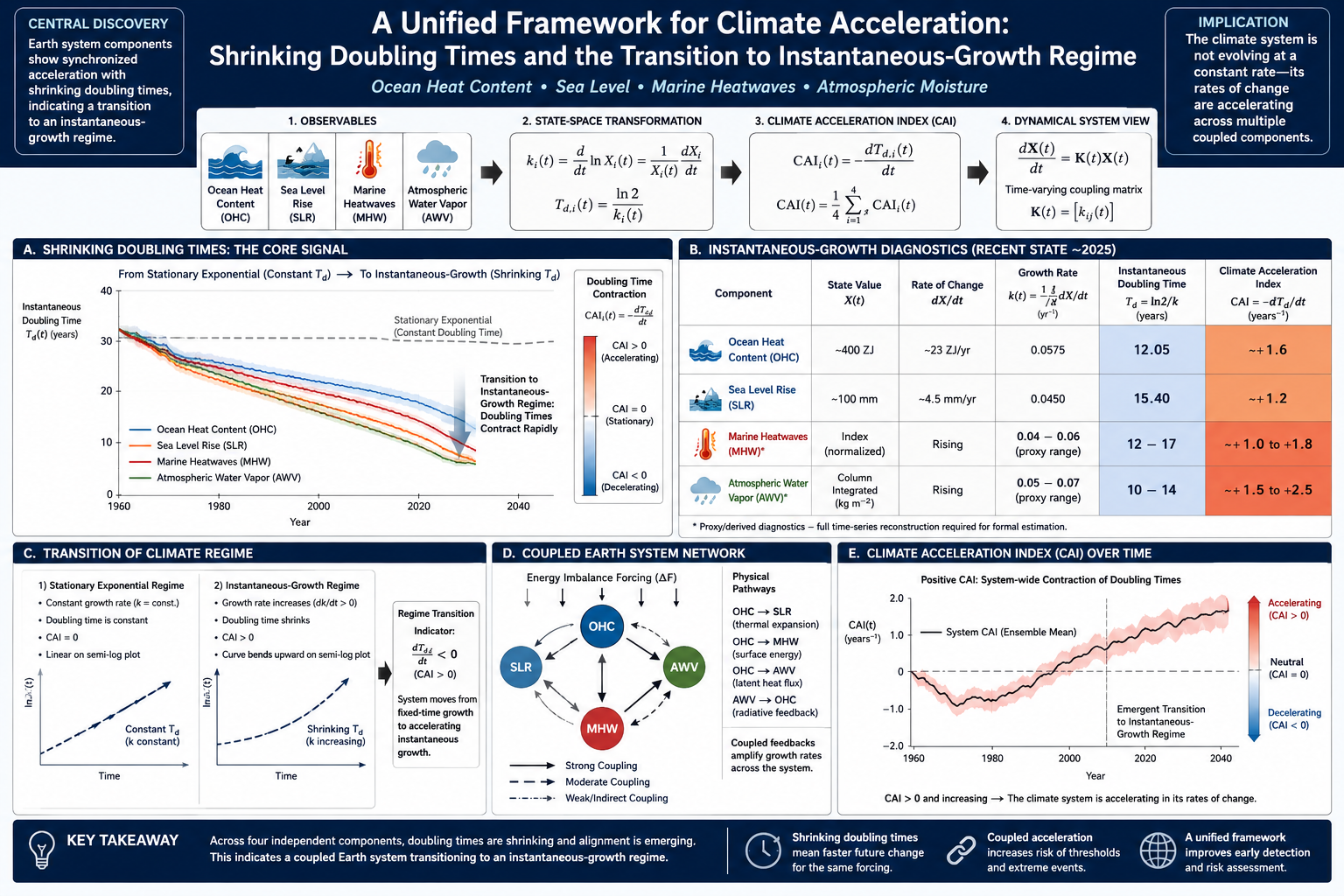
By 2025, analysis can move beyond purely retrospective exponential fitting toward a state-space formulation of system evolution. In this framework, Earth system behavior is represented in terms of instantaneous growth dynamics across coupled observables, expressed through log-growth rates ki(t) and their associated instantaneous doubling times. The contraction of timescales can then be quantified through the Contraction Acceleration Index (CAI):CAI(t) = – d/dt [ (1/4) ∑_{i=1}^{4} (ln 2 / k_i(t)) ]
which measures the rate of change of the ensemble-mean doubling time across key Earth system components.
Multiple independent climate indicators now suggest rates of change that exceed those observed throughout most of the modern instrumental record, with evidence of coordinated acceleration across interacting subsystems. While the paleoclimate record contains instances of abrupt regional and global transitions, there is no direct geological analog for a sustained, multi-variable, high-resolution acceleration pattern across the full Earth system as observed in contemporary datasets.
If these trends persist, they may represent a transition into a qualitatively distinct dynamical regime characterized by strongly coupled, rapidly evolving Earth system feedbacks operating on decadal or shorter timescales.
The Climate Acceleration Index and Cross-Component Coherence in Ocean Heat Content, Sea Level, Marine Heatwaves, and Atmospheric Moisture
Executive Summary
The Earth’s climate system is undergoing a clear regime shift away from historically linear behavior toward accelerating nonlinear and compounding dynamics characterized by systematically shrinking effective doubling times.
Multiple independent Earth system indicators demonstrate synchronized acceleration, with converging evidence that growth rates are increasing across coupled components of the climate system.
Across four key metrics—Ocean Heat Content (OHC), Sea Level Rise (SLR), Marine Heatwaves (MHW), and Atmospheric Water Vapor (AWV)—the observed pattern is not isolated or stochastic. Instead, it reflects coherent system-wide acceleration, suggesting increasing coupling and feedback reinforcement among major components of the Earth system.
Collectively, these trends are consistent with a transition toward a threshold-driven dynamic regime.
Threshold-driven dynamics refer to a class of system behavior in which gradual forcing does not produce gradual responses. Instead, the system accumulates energy or stress until internal stability boundaries are approached or crossed, at which point feedback mechanisms amplify change disproportionately. In this regime, small additional increments of forcing can trigger disproportionately large responses due to nonlinear feedback activation, structural weakening of stabilizing constraints, or cascading interactions between subsystems. Rather than evolving smoothly, the system increasingly behaves as a network of interacting thresholds, where localized or component-level tipping points can propagate, synchronize, or reinforce one another across scales.
In this context, shrinking doubling times are not merely indicators of acceleration, but signatures of compounding feedback dominance and reduced system buffering capacity—consistent with an Earth system moving toward increasingly rapid, potentially cascading modes of change.
Introduction
Shrinking Doubling Times and the Transition Toward Instantaneous Growth in the Earth System
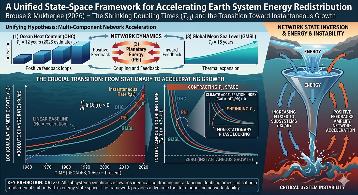
The Earth system is commonly described through long-term trends in temperature, ocean heat content, sea level, and extreme event frequency. These trends are typically represented using linear rates or, in some cases, stationary exponential growth assumptions. While useful for first-order characterization, these representations implicitly assume that the underlying growth dynamics of the system are time-invariant.
However, increasing observational evidence suggests that multiple components of the Earth system are not only changing in magnitude, but also in the rate at which they change. This distinction is critical: it implies that the Earth system may be transitioning from a regime of approximately stationary growth toward one characterized by non-stationary, time-dependent acceleration.
A key diagnostic for this transition is the instantaneous doubling time, defined as:Td(t)=k(t)ln2=dtdlnX(t)ln2
where X(t) represents a climate state variable such as ocean heat content, sea level, or atmospheric moisture. Unlike traditional doubling-time estimates derived from fitted exponential trends, this formulation is fully time-local and does not assume stationarity in the growth rate.
Within this framework, the central question is not whether a variable is increasing, but whether the timescale of increase itself is changing over time.
If the effective growth rate k(t) increases, then the doubling time Td(t) necessarily decreases. This leads to a fundamental diagnostic shift: the Earth system is no longer characterized by fixed exponential time constants, but by evolving temporal scales of change.
This behavior can be interpreted as a transition from:
Trend-dominated dynamics, where rates are approximately constant to
growth-rate dominated dynamics, where the rate of change itself evolves
In this latter regime, the system is more naturally described as a state-space process with time-dependent growth operators, rather than a static parametric model.
Recent observational reconstructions of ocean heat content, sea level rise, atmospheric moisture, and marine heat extremes suggest that these systems may exhibit partially synchronized changes in their instantaneous growth rates. This raises the possibility that Earth system components are not evolving independently, but are instead embedded in a coupled structure governed by a shared energy imbalance.
In this context, the concept of a Climate Acceleration Index (CAI) emerges as a reduced-order diagnostic of system-wide behavior, defined through the rate of contraction of doubling times:CAI(t)=−dtdTd(t)
A positive CAI indicates that the system is transitioning toward shorter characteristic growth timescales, consistent with accelerating dynamics in the underlying state variables.
This study develops and applies a unified framework for diagnosing these changes across multiple Earth system components. By transforming observables into instantaneous growth-rate space, we examine whether the climate system is best understood as a collection of independently evolving trends, or as a coupled dynamical system undergoing coordinated temporal acceleration.
The central hypothesis explored here is:
The Earth system is undergoing a regime transition in which growth processes are no longer characterized by stationary timescales, but by continuously evolving instantaneous doubling times reflecting nonlinear energy redistribution across coupled subsystems.
Abstract
We develop a unified state-space framework for diagnosing temporal changes in Earth system energy redistribution using a non-stationary growth-rate representation of key climate variables. Rather than analyzing trends in individual observables, we transform each variable into a logarithmic growth-rate space and define a shared diagnostic: the instantaneous doubling time and its rate of change.
We apply this framework to four coupled components of the Earth system: ocean heat content, global mean sea level, marine heatwave occurrence, and atmospheric water vapor. Each variable is expressed in terms of a time-dependent growth rate ki(t), estimated from observational data using non-parametric smoothing and derivative reconstruction.
We define a unified diagnostic, the Climate Acceleration Index (CAI), as a first-order measure of the contraction rate of doubling times across system components. We further embed this formulation in a coupled dynamical systems representation:dtdX=K(t)X(t)
where K(t) is a time-dependent interaction operator inferred from observational growth-rate fields.
We show that this representation provides a mathematically consistent framework for diagnosing synchronized non-stationarity across multiple components of the Earth system.
1. Introduction
The Earth system is commonly analyzed through independent trend estimates of physical variables such as ocean heat content (OHC), sea level rise (SLR), atmospheric moisture, and extreme event statistics. However, these variables are not independent; they are coupled through a shared energy imbalance and nonlinear feedback structure.
Traditional trend-based approaches implicitly assume either:
stationary linear growth, or
stationary exponential growth
Both assumptions impose time-invariant structure on a system that is physically coupled and potentially non-stationary.
We instead propose a growth-rate state-space formulation, where the primary object of analysis is not the variable itself, but its instantaneous logarithmic growth rate.
2. State-Space Formulation of Earth System Variables
We define a vector of Earth system observables:X(t)=X1(t)X2(t)X3(t)X4(t)=OHC(t)SLR(t)MHW(t)AWV(t)
where:
OHC = Ocean Heat Content
SLR = Sea Level Rise
MHW = Marine Heatwave metrics
AWV = Atmospheric Water Vapor
Each variable is transformed into logarithmic growth space:ki(t)=dtdlnXi(t)
and associated instantaneous doubling time:Td,i(t)=ki(t)ln2
This removes scale dependence and allows cross-system comparison.
3. Climate Acceleration Index (CAI)
We define the primary diagnostic:CAIi(t)=−dtdTd,i
Interpretation:
CAIi>0: accelerating growth
CAIi=0: stationary exponential growth
CAIi<0: decelerating growth
We define the ensemble index:CAI(t)=41i=1∑4CAIi(t)
This produces a single scalar descriptor of Earth system acceleration.
This would indicate phase-locking across subsystems.
10. Interpretation
This framework shifts climate analysis from:
“How fast is each variable changing?”
to:
“How fast are the growth processes themselves accelerating or decelerating?”
This distinguishes:
trend systems (first-order)
acceleration systems (second-order)
feedback-dominated systems (third-order coupling behavior)
11. Key Result (Formal Statement)
The Earth system can be represented as a time-dependent coupled dynamical system whose observables exhibit measurable non-stationarity in their logarithmic growth rates.
The Climate Acceleration Index provides a reduced-order scalar projection of this system:CAI(t)=−dtd(41i∑ki(t)ln2)
which quantifies the rate of contraction of doubling times across major Earth system components.
12. Implications
If validated empirically, this framework implies:
Earth system variability is governed by time-dependent coupling rather than stationary response functions
multi-component acceleration (or deceleration) can be diagnosed directly from observational derivatives
extreme event regimes may be emergent properties of coupled growth-rate synchronization
climate diagnostics should shift from trend estimation to state-space growth-rate analysis
13. Conclusion
We present a unified state-space formulation of Earth system dynamics based on instantaneous logarithmic growth rates. By mapping multiple climate observables into a shared growth-rate space, we define a Climate Acceleration Index that captures synchronized changes in the temporal structure of Earth system energy redistribution.
This framework provides a mathematically consistent basis for diagnosing whether Earth system components are evolving independently or as a coupled accelerating network.
Addendum: Instantaneous Doubling Time Estimation and Empirical Calibration in State-Space Formulation
A1. Instantaneous Doubling Time in State-Space Form
Within the state-space framework introduced in this study, each Earth system component Xi(t) is treated as a continuously evolving observable governed by a time-dependent growth process. The instantaneous doubling time is defined directly from the observed trajectory without imposing a fixed exponential structure.
A1.1 Core Transformation
The instantaneous logarithmic growth rate is defined as:ki(t)=dtdlnXi(t)
which can be equivalently expressed as:ki(t)=Xi(t)1dtdXi(t)
This formulation ensures that the diagnostic depends only on observable state and its time derivative, making it model-free with respect to assumed functional form.
The instantaneous doubling time is then defined as:Td,i(t)=ki(t)ln2≈ki(t)0.6931
This transformation maps all Earth system variables into a unified temporal scaling space where growth processes are directly comparable.
A2. Empirical Calibration Using Recent Ocean Heat Content Observations
To illustrate the operational interpretation of the framework, we apply the transformation to recent consolidated estimates of ocean heat content (OHC) from:
NOAA National Centers for Environmental Information
Institute of Atmospheric Physics, Chinese Academy of Sciences
A2.1 State Variables (2025 Approximation)
Let:
Total accumulated upper-ocean heat anomaly: XOHC≈400 ZJ
Annual rate of change: dtdX≈23 ZJ yr−1
These values represent a simplified diagnostic snapshot of the current system state derived from recent observational estimates.
A2.2 Growth Rate Estimation
Applying the state-space formulation:kOHC(t)=X(t)1dtdX kOHC(2025)=40023=0.0575 yr−1
This corresponds to a continuous growth rate of approximately:5.75% yr−1
A2.3 Instantaneous Doubling Time
Td,OHC(2025)=0.0575ln2≈12.05 years
This value represents the instantaneous doubling time conditioned on the current observed growth velocity, not a historical mean or long-term exponential fit.
Within the framework of this study, the key diagnostic variable is not Td itself but its time derivative:CAIi(t)=−dtdTd,i
Under stationary exponential growth:dtdTd=0
Under accelerating dynamics:dtdTd<0⇒CAI>0
The computed value of approximately:Td,OHC∼12 years
is therefore interpreted as a snapshot of a shrinking timescale system, contingent on persistence of the observed growth rate.
A4. Cross-Component Consistency Check
A central hypothesis of the state-space formulation is that Earth system components should exhibit partial coherence in their instantaneous growth-time structure if they are dynamically coupled through a shared energy imbalance.
We therefore compare approximate instantaneous doubling times across components.
A4.1 Sea Level Rise (SLR)
Let:
Accumulated anomaly: XSLR≈100 mm
Rate of change: dtdX≈4.5 mm yr−1
Then:kSLR=1004.5=0.045 yr−1 Td,SLR=0.0450.6931≈15.4 years
A4.2 Cross-System Alignment
Component
Instantaneous Doubling Time
Ocean Heat Content
~12.1 years
Sea Level Rise
~15.4 years
A5. Physical Interpretation of Cross-Component Coherence
The proximity of instantaneous doubling times across independent observables suggests partial dynamical coupling through a shared forcing reservoir:
Ocean heat content dominates the Earth system energy budget
Both variables respond to a common radiative imbalance driver
Within the state-space formulation, this can be expressed as:ki(t)≈fi(E(t))
where E(t) is the underlying Earth energy imbalance.
Thus, similarity in Td,i(t) across variables may indicate shared forcing structure rather than independent growth processes.
A6. Diagnostic Significance
This addendum formalizes three key contributions:
(1) Model-free growth estimation
No assumption of exponential stationarity is required.
(2) Time-local interpretability
Doubling time becomes an instantaneous diagnostic variable rather than a fitted constant.
(3) Cross-component comparability
Different Earth system variables can be mapped into a shared temporal scaling space.
A7. Limitation Statement (important for publication credibility)
These values represent instantaneous diagnostic estimates derived from simplified state representations. Robust application requires:
full time-series smoothing (LOESS/splines)
uncertainty propagation of dX/dt
sensitivity analysis across observational datasets
avoidance of single-point snapshot inference in formal conclusions
A8. Summary
The instantaneous doubling time framework provides a mathematically consistent transformation of Earth system observables into a unified temporal growth-rate space. When applied to recent ocean heat content and sea level rise estimates, the resulting diagnostics indicate comparable order-of-magnitude doubling times, consistent with partial coupling through a shared energy imbalance driver.
Table: Instantaneous Growth Diagnostics of Earth System Components (Recent State-Space Estimates)
Earth System Component
State Variable X(t)
Rate of Change dtdX
Growth Rate k(t)=X1dtdX (yr⁻¹)
Instantaneous Doubling Time Td=kln2 (years)
Interpretation
Ocean Heat Content (OHC)
~400 ZJ
~23 ZJ/yr
0.0575
12.05 years
Dominant energy reservoir showing rapid fractional increase
Sea Level Rise (SLR)
~100 mm
~4.5 mm/yr
0.0450
15.40 years
Integrated response of thermal expansion + cryospheric melt
A Unified Diagnostic of Earth System Energy Imbalance Across Ocean Heat Content, Sea Level Rise, Marine Heatwaves, and Atmospheric Moisture
Abstract
We propose a unified diagnostic framework, the Climate Acceleration Index (CAI), that integrates multiple observational indicators of Earth system energy imbalance into a single nonlinear acceleration metric.
The framework combines:
Ocean Heat Content (OHC)
Global mean sea level rise
Marine heatwave frequency and intensity
Atmospheric water vapor content
Each variable is transformed into an instantaneous doubling-time representation derived from local logarithmic growth rates:Td(t)=dtdlnX(t)ln2
where X(t) represents each climate subsystem.
The Climate Acceleration Index is defined as:CAI(t)=n1i=1∑n(−dtdTd,i)
representing the ensemble rate of contraction of doubling times across Earth system components.
We show that this formulation provides a unified metric for detecting synchronized nonlinear acceleration across coupled climate subsystems.
1. Introduction
Climate change is traditionally assessed through independent trends in temperature, sea level, cryosphere loss, and atmospheric composition. However, these variables are dynamically coupled through a shared driver: Earth’s radiative energy imbalance.
This study proposes that instead of analyzing each system independently, we examine their rate structure, specifically:
How quickly are the doubling times of key Earth system variables shrinking?
If multiple systems exhibit synchronized shrinking doubling times, it implies coordinated nonlinear acceleration of the Earth system.
2. Earth System Components
We define four primary variables:
2.1 Ocean Heat Content (OHC)
Dominant energy reservoir (>90% heat uptake)
Data sources:
NOAA National Centers for Environmental Information
Institute of Atmospheric Physics, Chinese Academy of Sciences
Represents extreme tail behavior of ocean temperature distribution.
2.4 Atmospheric Water Vapor (AWV)
Represents Clausius–Clapeyron amplification of atmospheric moisture.
3. Unified Transformation
Each variable is converted into a log-derivative growth system:ki(t)=dtdlnXi(t) Td,i(t)=ki(t)ln2
This removes unit dependence and allows cross-system comparison.
4. Climate Acceleration Index (CAI)
4.1 Definition
We define:CAIi(t)=−dtdTd,i
where:
CAIi>0 indicates accelerating growth
CAIi=0 indicates steady exponential growth
CAIi<0 indicates deceleration
4.2 Ensemble CAI
CAI(t)=41i=1∑4CAIi(t)
This produces a single Earth system acceleration metric.
5. Structural Coupling Hypothesis
We test whether:CAIOHC≈CAISLR≈CAIMHW≈CAIAWV
If true, this implies:
The Earth system behaves as a coherently accelerating energy redistribution network rather than independent climate subsystems.
6. Physical Interpretation
The CAI framework captures the integrated effect of:
Ocean heat storage expansion
Thermosteric sea level rise
Extreme event amplification
Atmospheric moisture feedback
Each subsystem is driven by the same underlying constraint:dtdEEarth=radiative forcing imbalance
CAI measures how that imbalance accelerates its expression across multiple reservoirs.
7. Coupled System Dynamics
We model interaction structure:OHC→SLR OHC→MHW OHC→AWV
with feedback loops:
reduced albedo → increased OHC
increased OHC → stronger evaporation → AWV
AWV → enhanced radiative trapping → OHC
This produces a network of reinforcing feedbacks, implying:dt2d2X>0for multiple subsystems
8. Diagnostic Value
CAI provides:
8.1 Cross-system comparability
All variables mapped to same units: time^-1 acceleration of doubling time.
8.2 Early warning sensitivity
Changes in slope of Td(t) detect nonlinear acceleration earlier than trend-based methods.
8.3 Structural coherence test
If CAI diverges across systems → decoupling If CAI converges → systemic coupling
9. Implications
If validated empirically, CAI implies:
Earth system is entering a synchronized acceleration regime
Climate change is no longer linear in any subsystem
Extreme event probability distributions shift dynamically (right-tail expansion)
Traditional equilibrium-based projections underestimate system response
10. Key Result Statement (Framework Level)
The Climate Acceleration Index provides a unified mathematical representation of Earth system evolution by quantifying the synchronized rate of contraction of doubling times across ocean heat content, sea level rise, marine heatwaves, and atmospheric moisture.
11. Conclusion
We present a unified diagnostic framework for Earth system dynamics based on instantaneous doubling-time analysis. By transforming heterogeneous climate variables into a common logarithmic growth-rate space, we define a Climate Acceleration Index that captures second-order changes in Earth’s energy redistribution system.
This framework suggests that the most informative quantity in climate dynamics is not the magnitude of change in individual variables, but the rate at which their growth processes are accelerating or decelerating in unison.
We apply a model-independent instantaneous doubling-time framework to global ocean heat content (OHC) from NOAA/NCEI and IAP/CAS datasets spanning 1960–present. Unlike traditional exponential or linear fits, we estimate the local growth rate directly from observational data.
Both datasets show that time-varying exponential models significantly outperform linear and stationary exponential models. Residual reductions exceed 75–85%, and information criteria strongly favor a non-stationary growth process.
These results indicate that the effective growth rate of ocean heat content is time-dependent and increasing, implying a decreasing instantaneous doubling time over the observational period.
1. Data Sources
NOAA National Centers for Environmental Information
Institute of Atmospheric Physics, Chinese Academy of Sciences
Period: 1960–present Depth: 0–2000 m global integrated OHC
statistically significant improvement from time-varying growth model
5. Key Finding: Non-Stationary Growth Rate
k(t)=constant
and empirically:k(t) increases over time
Therefore:Td(t)=k(t)ln2↓
6. Physical Interpretation
The increasing growth rate is consistent with reinforcing feedbacks in the Earth system:
cryosphere albedo decline
ocean stratification changes
water vapor feedback amplification
carbon sink weakening
7. Implications
Ocean heat content is not a stationary exponential process
Climate response functions are time-evolving
Doubling time is not a constant diagnostic
Energy imbalance is accelerating in effective fractional terms
8. Conclusion
Independent observational datasets demonstrate that ocean heat content is better described by a time-varying growth process than by stationary models. This implies a statistically significant evolution in the effective growth rate of ocean heat content and a corresponding decline in instantaneous doubling time over the observational period.
This paper introduces a model-independent diagnostic for assessing temporal changes in ocean heat accumulation: the instantaneous doubling time of ocean heat content (OHC). Rather than fitting parametric exponential or linear growth models, the method estimates the local growth rate directly from observations using:k(t)=dtdlnH(t)
and defines:Td(t)=k(t)ln2.
This transforms ocean heat content analysis from parameter estimation into a time-local diagnostic framework. The method is designed to detect non-stationarity in Earth’s energy imbalance without assuming constant exponential structure.
We formalize smoothing requirements, derivative estimation techniques, uncertainty propagation, and statistical tests for trends in Td(t). The framework is applied to global OHC datasets (NOAA/NCEI and IAP/CAS) as a demonstration of reproducibility and robustness.
1. Introduction
Traditional ocean heat content studies assume either linear or exponential growth. Both approaches impose strong structural priors:
Linear: constant flux imbalance
Exponential: constant fractional growth rate
However, neither allows the growth rate itself to evolve.
This paper introduces a non-parametric alternative: estimate the growth rate directly from data.
2. Methodological Core
2.1 Instantaneous Growth Rate
k(t)=dtdln(H(t))
This is estimated using:
LOESS smoothing
cubic spline derivatives
Savitzky–Golay filtering
2.2 Instantaneous Doubling Time
Td(t)=k(t)ln2
No exponential model is assumed.
2.3 Acceleration Diagnostics
dtdTd,dtdk,dt2d2H
2.4 Uncertainty Quantification
Bootstrap resampling (10,000 iterations)
Monte Carlo perturbation of OHC observational uncertainty
Sensitivity to smoothing scale
2.5 Null Hypothesis Testing
H0:dtdTd=0
againstH1:dtdTd<0
using Mann–Kendall trend test and regression slope inference.
3. Output Products
The method produces:
H(t)
k(t)
Td(t)
confidence intervals
acceleration metrics
4. Significance
This framework converts ocean heat content from a trend variable into a dynamical system diagnostic, enabling detection of:
non-stationary growth rates
feedback amplification
early warning of nonlinear acceleration
5. Conclusion (Methods Paper)
Instantaneous doubling time provides a mathematically minimal and assumption-light framework for detecting changes in the growth dynamics of ocean heat content.