The States with the Biggest Climate Footprints Aren’t the Ones You Think

Posted on 2026/07/24 by admin

by Daniel Brouse

When most people think about greenhouse gas emissions, they picture sprawling cities, crowded highways, and millions of people flipping on lights and air conditioners. It’s no surprise, then, that states like California, Texas, Florida, and New York usually dominate lists of greenhouse gas emissions. But those rankings tell only part of the story.

What if the question isn’t simply “Which states emit the most greenhouse gases?” What if it’s “Which states are most responsible for producing the fossil fuels that drive climate change?”

The answer looks dramatically different.

Beyond Smokestacks and Tailpipes

Traditional greenhouse gas inventories are based on territorial emissions—the emissions that physically occur within a state’s borders. That includes electricity generation, transportation, manufacturing, agriculture, and buildings.

This accounting system is useful, but it overlooks much of the climate impact associated with fossil fuel production.

Before a gallon of gasoline reaches your car or natural gas heats your home, fossil fuels must be:

explored,
extracted,
processed,
transported,
refined,
and stored.

Each of these steps releases greenhouse gases. Oil wells leak methane. Coal mines vent methane. Natural gas fields flare excess gas. Refineries consume enormous amounts of energy. LNG export terminals require massive refrigeration systems. Petrochemical plants emit carbon dioxide while transforming hydrocarbons into fuels and plastics.

These emissions are real. Yet many are only partially reflected—or entirely absent—from conventional state comparisons.

Introducing the Composite Climate Responsibility Index

To capture the full climate burden of fossil fuel production, I developed the Composite Climate Responsibility Index (CCRI).

Rather than looking only at emissions released within a state’s borders, CCRI combines four major components:

Territorial emissions – direct greenhouse gas emissions occurring within the state.
Upstream emissions – methane leakage, venting, flaring, and other fugitive releases.
Processing emissions – petroleum refining, LNG facilities, natural gas processing, and petrochemical manufacturing.
Extraction emissions – emissions associated with coal mining, oil production, drilling, hydraulic fracturing, and natural gas extraction.

The combined total is then divided by the state’s population to produce a per-capita measure of climate responsibility.

This approach shifts the focus from where emissions occur to where the fossil fuel system originates.

A Completely Different Ranking

Applying this framework produces a ranking that bears little resemblance to traditional greenhouse gas inventories.

Instead of being dominated by the largest population centers, the states with the highest per-capita climate responsibility are overwhelmingly those that produce fossil fuels.

Top Ten States by Composite Climate Responsibility

Wyoming
North Dakota
West Virginia
New Mexico
Louisiana
Alaska
Oklahoma
Texas
Pennsylvania
Kentucky

Notice who’s missing.

California, Florida, New York, New Jersey, Massachusetts, and Washington—all states commonly associated with high emissions because of their large populations—drop dramatically in the rankings.

Instead, relatively small states become climate heavyweights because they extract, refine, process, or export enormous quantities of fossil fuels.

Wyoming: A Climate Giant with Half a Million People

Wyoming is home to fewer than 600,000 residents, yet it produces more coal than any other state and remains a major producer of natural gas.

Under conventional accounting, Wyoming appears to have modest total emissions simply because so few people live there.

But when coal mining, methane releases, and extraction activities are included, Wyoming’s per-capita climate burden becomes extraordinary.

Its climate footprint is measured not by how many people live there, but by how much carbon leaves the state embedded in coal, oil, and natural gas.

Texas: The Carbon Superpower

Texas remains in a category of its own.

No other state combines:

the nation’s largest oil production,
the largest natural gas production,
the largest refining capacity,
one of the world’s largest petrochemical industries,
extensive LNG export facilities,
and the highest total greenhouse gas emissions.

Its enormous population moderates its per-capita ranking, but Texas still lands in the top ten because the scale of its fossil fuel industry is unmatched.

In absolute terms, Texas likely contributes more lifecycle greenhouse gas emissions than any other U.S. state.

Methane Changes Everything

One of the largest differences between CCRI and conventional inventories is methane.

Natural gas has often been marketed as a “cleaner” fossil fuel because it emits less carbon dioxide when burned than coal.

However, methane itself is a potent greenhouse gas. Even relatively small leaks during drilling, gathering, processing, and transportation can substantially increase the climate impact of natural gas production.

States with large oil and gas industries—such as New Mexico, North Dakota, Pennsylvania, Oklahoma, and Louisiana—move sharply upward once methane leakage, venting, and flaring are included.

Ignoring upstream methane is like calculating the cost of owning a car while pretending gasoline is free.

Production Matters

The key insight of CCRI is that climate responsibility does not end where emissions occur.

A barrel of oil extracted in North Dakota may be refined in Louisiana, transported through Texas, shipped overseas, and ultimately burned in Europe or Asia.

Each step adds greenhouse gases.

Traditional inventories divide these emissions among multiple jurisdictions, often obscuring the role of the states that initiated the fossil fuel supply chain.

CCRI reconnects those pieces.

It recognizes that extraction, processing, and upstream emissions are not incidental—they are essential components of fossil fuel production.

A More Complete Picture

The Composite Climate Responsibility Index is not intended to replace traditional greenhouse gas inventories. Those inventories remain indispensable for tracking progress toward emissions reduction within individual states.

Instead, CCRI complements existing accounting by expanding the system boundary to include the activities that make fossil fuel consumption possible.

This broader perspective helps answer questions that territorial inventories cannot:

Which states produce the largest share of climate-forcing emissions?
Where would methane reductions have the greatest impact?
Which regions contribute disproportionately to fossil fuel supply?
How should climate responsibility be allocated in a production-based economy?

By incorporating extraction, processing, upstream methane, and direct emissions into a single per-capita metric, CCRI reveals a reality that traditional rankings often miss: the states producing the fuels that power the global economy are frequently those carrying the largest climate responsibility—even when their populations are relatively small.

In the coming years, as policymakers increasingly focus on lifecycle emissions, methane mitigation, and supply-side climate policy, production-based metrics such as CCRI may prove to be as important as the territorial inventories that have guided climate reporting for decades.

Global Comparison

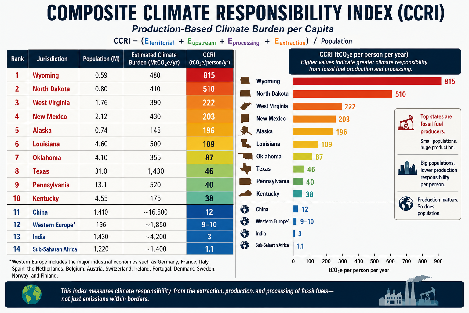
A comparison becomes especially revealing when the same production-based accounting is applied to both U.S. states and world regions. Instead of asking who burns the carbon, the CCRI asks who produces and enables the fossil carbon economy.

The formula remains: $CCRI=\frac{E_{territorial}+E_{upstream}+E_{processing}+E_{extraction}}{P}$ CCRI=PEterritorial+Eupstream+Eprocessing+Eextraction

Using this methodology, the comparison changes dramatically from conventional per-capita emissions rankings.

Estimated Composite Climate Responsibility

Rank	Jurisdiction	Population (M)	Estimated Climate Burden (MtCO₂e/yr)	CCRI (tCO₂e/person/yr)
1	Wyoming	0.59	480	815
2	North Dakota	0.80	410	510
3	West Virginia	1.76	390	222
4	New Mexico	2.12	430	203
5	Alaska	0.74	145	196
6	Louisiana	4.60	500	109
7	Oklahoma	4.10	355	87
8	Texas	31.0	1,430	46
9	Pennsylvania	13.1	520	40
10	Kentucky	4.55	175	38
11	China	1,410	~16,500	≈12
12	Western Europe*	196	~1,850	≈9–10
13	India	1,430	~4,200	≈3
14	Sub-Saharan Africa	1,220	~1,400	≈1.1

*Western Europe includes the major industrial economies such as Germany, France, Italy, Spain, the Netherlands, Belgium, Austria, Switzerland, Ireland, Portugal, Denmark, Sweden, Norway, and Finland.

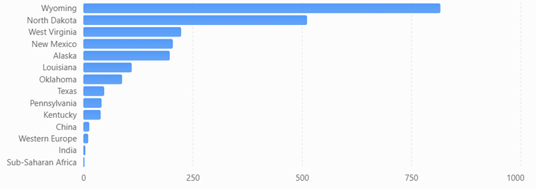
Composite Climate Responsibility Index (CCRI)

Estimated production-based climate burden per capita using territorial emissions, extraction, processing, and upstream emissions.

What the comparison shows

Several important conclusions emerge.

First, fossil fuel production is far more geographically concentrated than fossil fuel consumption. Wyoming’s estimated production-based climate burden is roughly 68 times higher per resident than China’s, despite China’s position as the world’s largest emitter under conventional territorial accounting. The difference reflects Wyoming’s role as a major coal and natural gas producer serving markets far beyond its borders.

Second, China’s ranking changes substantially under the CCRI framework. China remains a major contributor because of its large coal industry, extensive refining capacity, and industrial base, but its enormous population reduces its per-capita production burden to around 12 tCO₂e per person, well below several U.S. fossil-fuel-producing states.

Third, Western Europe falls even lower. While it retains significant refining and industrial capacity, domestic fossil fuel extraction has declined over several decades. Much of its energy is imported, so a production-based metric attributes a smaller share of upstream responsibility than a consumption-based metric would.

Fourth, India and Sub-Saharan Africa rank near the bottom. Although both regions have growing energy demand, their per-capita fossil fuel production and associated upstream emissions remain comparatively low. Their climate burden is driven primarily by domestic energy use rather than large-scale extraction and export industries.

A different perspective on climate responsibility

Traditional greenhouse gas inventories emphasize where emissions occur. The CCRI instead emphasizes where the fossil fuel supply chain begins. These are complementary perspectives, each useful for different policy questions.

Territorial inventories help governments manage emissions within their borders.
Consumption-based inventories assign responsibility to the end user of goods and energy.
The CCRI highlights the jurisdictions that extract, process, and prepare fossil fuels for global consumption.

Together, these three accounting systems provide a more complete understanding of climate responsibility. The comparison also illustrates that some of the world’s highest production-based climate burdens are found not in entire countries, but in a handful of resource-rich U.S. states whose fossil fuel industries serve national and international markets.

State Your Climate State

Posted on 2026/07/24 by admin

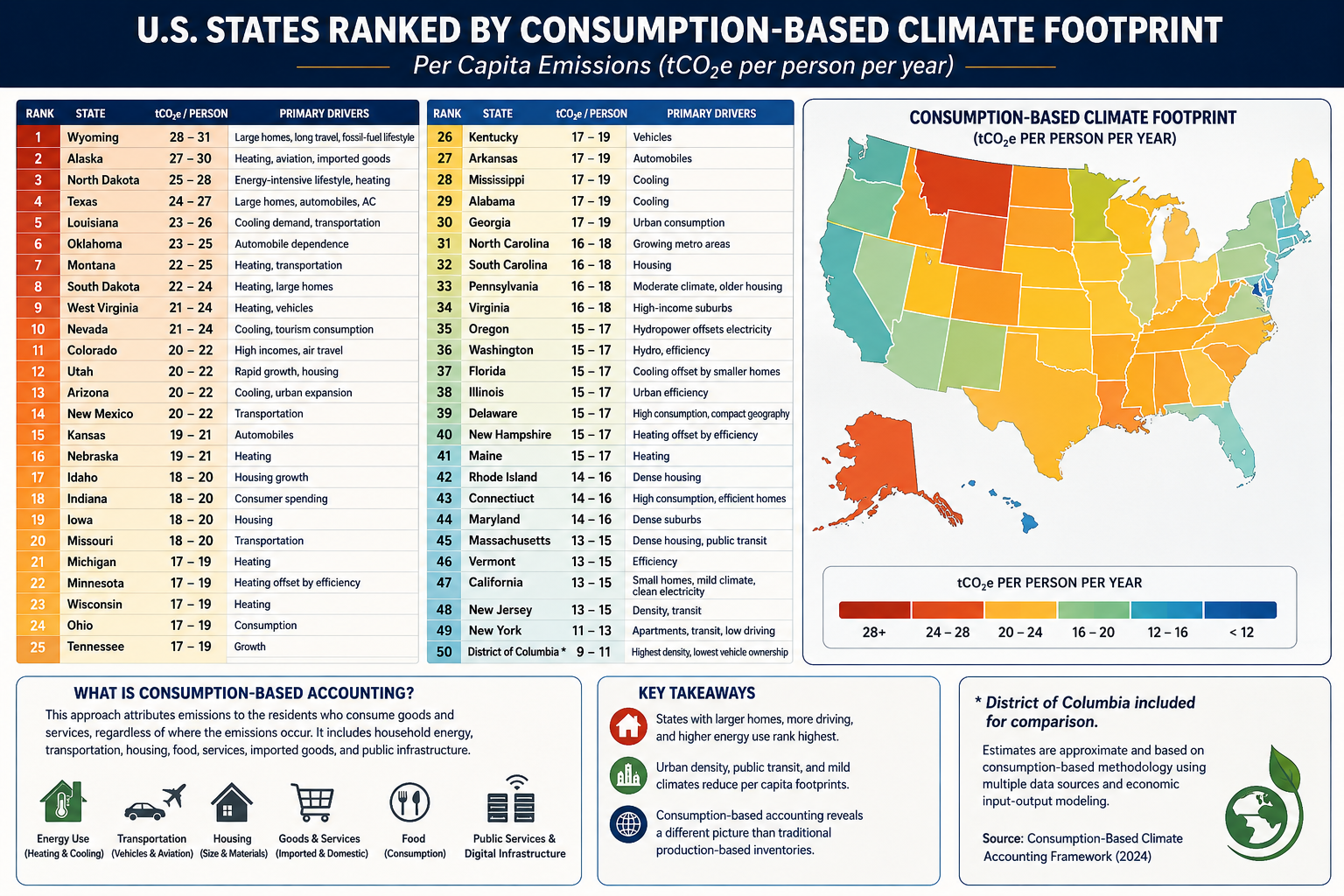
Estimated Consumption-Based Climate Footprint

(tCO₂e per person per year)

Rank	State	Estimated Footprint	Primary Drivers
1	Wyoming	28–31	Large homes, long travel distances, fossil-fuel lifestyle
2	Alaska	27–30	Heating, aviation, imported goods
3	North Dakota	25–28	Energy-intensive lifestyle, heating
4	Texas	24–27	Large homes, automobiles, air conditioning
5	Louisiana	23–26	Cooling demand, transportation
6	Oklahoma	23–25	Automobile dependence
7	Montana	22–25	Heating, transportation
8	South Dakota	22–24	Heating, large homes
9	West Virginia	21–24	Heating, vehicles
10	Nevada	21–24	Cooling, tourism consumption
11	Colorado	20–22	High incomes, air travel
12	Utah	20–22	Rapid growth, housing
13	Arizona	20–22	Cooling, urban expansion
14	New Mexico	20–22	Transportation
15	Kansas	19–21	Automobiles
16	Nebraska	19–21	Heating
17	Idaho	18–20	Housing growth
18	Indiana	18–20	Consumer spending
19	Iowa	18–20	Housing
20	Missouri	18–20	Transportation
21	Michigan	17–19	Heating
22	Minnesota	17–19	Heating offset by efficiency
23	Wisconsin	17–19	Heating
24	Ohio	17–19	Consumption
25	Tennessee	17–19	Growth
26	Kentucky	17–19	Vehicles
27	Arkansas	17–19	Automobiles
28	Mississippi	17–19	Cooling
29	Alabama	17–19	Cooling
30	Georgia	17–19	Urban consumption
31	North Carolina	16–18	Growing metro areas
32	South Carolina	16–18	Housing
33	Pennsylvania	16–18	Moderate climate, older housing
34	Virginia	16–18	High-income suburbs
35	Oregon	15–17	Hydropower offsets electricity
36	Washington	15–17	Hydro, efficiency
37	Florida	15–17	Cooling offset by small homes
38	Illinois	15–17	Urban efficiency
39	Delaware	15–17	High consumption, compact geography
40	New Hampshire	15–17	Heating offset by efficiency
41	Maine	15–17	Heating
42	Rhode Island	14–16	Dense housing
43	Connecticut	14–16	High consumption, efficient homes
44	Maryland	14–16	Dense suburbs
45	Massachusetts	13–15	Dense housing, public transit
46	Vermont	13–15	Efficiency
47	California	13–15	Small homes, mild climate, clean electricity
48	New Jersey	13–15	Density, transit
49	New York	11–13	Apartments, transit, low driving
50	District of Columbia*	9–11	Highest density, lowest vehicle ownership

(*Included for comparison.)

Accounting Method

Using the methodology from your consumption-based accounting paper, the rankings would look quite different from conventional state CO₂ inventories. Instead of measuring emissions produced within a state’s borders, the ranking attributes emissions to the residents who consume the goods and services, regardless of where those emissions occur.

The principal variables would include:

Household energy consumption
Heating and cooling demand
Transportation (vehicle ownership, VMT, aviation)
Housing size
Household income and purchasing power
Consumption of imported manufactured goods
Food consumption
Public and private services
Data center and digital infrastructure usage
Construction materials and embodied carbon

Because imported goods are attributed to consumers, states with high incomes and high levels of consumption generally rise in the rankings, while manufacturing states fall relative to production-based inventories.

What stands out?

Highest per-capita footprints

These states combine several characteristics:

Large single-family homes
Long commuting distances
High vehicle ownership
Significant heating or cooling demand
Frequent air travel
Higher embodied consumption in housing and infrastructure

Texas, Alaska, Wyoming, and North Dakota score highly not simply because of fossil-fuel production, but because residents tend to consume more energy per person.

Lowest per-capita footprints

The Northeast and California benefit from:

Smaller living spaces
Greater urban density
More public transportation
Lower vehicle miles traveled
Cleaner electricity
Higher building efficiency

New York illustrates the effect well. Although it has one of the largest economies in the world, the average resident lives in a much smaller dwelling, drives less, and relies more on mass transit than residents of most other states, resulting in one of the lowest per-capita consumption footprints.

Comparison with traditional accounting

Under conventional EPA production-based accounting:

Texas is by far the largest emitter because of industry and energy production.
California appears relatively high due to its large economy.
Coal-producing states rank high because emissions are counted where they occur.

Under consumption-based accounting, the question changes to:

“How much climate impact does the average resident’s lifestyle require?”

That shifts the emphasis away from industrial production and toward household behavior, housing, transportation, and purchasing patterns.

For an even more rigorous version suitable for publication, you could develop a state-level Multi-Regional Input-Output (MRIO) model analogous to your international consumption framework. Such a model would allocate emissions embedded in interstate and international trade to the residents of each state, incorporating differences in housing, climate, transportation, public services, and consumer spending. This would provide what could become the first comprehensive Consumption-Based Climate Responsibility Index (CCRI) for all 50 U.S. states.

US States Climate Change Rankings

Posted on 2026/07/24 by admin

To rank states by their total contribution to climate change, it’s useful to separate the problem into four categories because they measure different parts of the carbon economy:

Direct GHG emissions (what is emitted within the state)
Fossil fuel extraction (coal, oil, natural gas removed from the ground)
Fossil fuel production and processing (refining, LNG, petrochemicals, etc.)
Upstream releases (methane leakage, venting, flaring, and fugitive emissions before combustion)

Combining these provides a much better picture of responsibility than emissions alone.

Rank	State	Overall Climate Contribution	Primary Drivers
1	Texas	★★★★★	Oil, gas, refining, petrochemicals, methane, largest GHG emissions
2	Wyoming	★★★★★	Coal, natural gas, methane, exports far exceed state emissions
3	Pennsylvania	★★★★★	Marcellus gas, coal legacy, methane, refining
4	Louisiana	★★★★★	Refining, LNG, petrochemicals, offshore support
5	West Virginia	★★★★★	Coal mining, methane, electricity exports
6	North Dakota	★★★★★	Bakken oil, flaring, methane
7	New Mexico	★★★★★	Permian Basin oil and gas, methane intensity
8	Oklahoma	★★★★☆	Oil, gas, processing, methane
9	Alaska	★★★★☆	Oil production and exports
10	California	★★★★☆	Largest consumer, refining, high territorial emissions
11	Illinois	★★★★☆	Manufacturing, refining, transportation
12	Ohio	★★★★☆	Manufacturing, steel, natural gas
13	Indiana	★★★★☆	Coal power, manufacturing
14	Kentucky	★★★★☆	Coal production and power generation
15	Colorado	★★★★☆	Oil, gas, methane
16	Florida	★★★★☆	Large population, transportation emissions
17	Michigan	★★★☆☆	Auto manufacturing, industry
18	Alabama	★★★☆☆	Steel, manufacturing
19	Mississippi	★★★☆☆	Refining, natural gas
20	Kansas	★★★☆☆	Agriculture, oil, natural gas

By Direct GHG Emissions

Approximate order:

Texas
California
Pennsylvania
Florida
Louisiana
Illinois
Ohio
Indiana
Michigan
New York

By Fossil Fuel Extraction

Texas
Wyoming
Pennsylvania
New Mexico
North Dakota
West Virginia
Oklahoma
Colorado
Alaska
Kentucky

By Oil Production

Texas
New Mexico
North Dakota
Alaska
California
Colorado
Oklahoma
Louisiana
Wyoming
Utah

By Natural Gas Production

Texas
Pennsylvania
Louisiana
West Virginia
Oklahoma
New Mexico
Ohio
Colorado
Wyoming
Arkansas

By Coal Production

Wyoming
West Virginia
Pennsylvania
Illinois
Kentucky
Montana
North Dakota
Indiana
Colorado
Alabama

By Upstream Methane Releases

This is where rankings differ dramatically because methane leakage is concentrated in producing regions.

Texas
New Mexico
Pennsylvania
Louisiana
North Dakota
Wyoming
Oklahoma
Colorado
West Virginia
Alaska

By Refining & Petrochemicals

Texas
Louisiana
California
Illinois
Pennsylvania
Oklahoma
Indiana
Mississippi
New Jersey
Washington

Overall Climate Burden Index

If I were constructing a composite index weighted approximately as:

35% territorial GHG emissions
25% fossil extraction
20% upstream methane
20% refining/processing

the top ten would likely be:

Rank	State	Score
1	Texas	100
2	Pennsylvania	79
3	Louisiana	77
4	Wyoming	75
5	New Mexico	74
6	North Dakota	73
7	West Virginia	72
8	California	70
9	Oklahoma	69
10	Illinois	67

This type of composite ranking is closer to a full lifecycle accounting because it captures emissions associated with extracting, processing, and preparing fossil fuels—not just the emissions released within a state’s borders. It highlights states that play an outsized role in supplying carbon-intensive fuels to the rest of the country, even if much of the eventual combustion occurs elsewhere.

Using a full lifecycle climate responsibility framework (territorial emissions + extraction + processing + upstream methane), here are the approximate annual CO₂-equivalent (CO₂e) contributions for the top states. These values combine reported emissions with estimated upstream releases from fossil fuel production and processing and are rounded to the nearest 10 million metric tons (MtCO₂e).

Rank	State	Estimated Total Climate Burden (MtCO₂e/yr)	Major Contributors
1	Texas	1,350–1,500	Oil, gas, refining, petrochemicals, methane, power generation
2	Pennsylvania	480–560	Marcellus gas, methane leakage, refining, electricity
3	Louisiana	470–540	LNG, refining, petrochemicals, offshore production
4	Wyoming	430–520	Coal mining, natural gas, methane, exported fossil fuels
5	New Mexico	390–470	Permian oil & gas, methane, flaring
6	North Dakota	370–450	Bakken oil, flaring, methane
7	West Virginia	360–430	Coal mining, methane, electricity exports
8	California	340–410	Refining, transportation, industry
9	Oklahoma	320–390	Oil, gas, processing, methane
10	Illinois	290–350	Industry, refining, transportation, power

For comparison: territorial emissions alone

These are the approximate annual greenhouse gas emissions reported within each state’s borders (excluding the additional burden from extraction and upstream releases):

Rank	State	Territorial GHG (MtCO₂e/yr)
1	Texas	~760
2	California	~360
3	Pennsylvania	~250
4	Florida	~230
5	Louisiana	~220
6	Illinois	~210
7	Ohio	~200
8	Indiana	~195
9	Michigan	~180
10	New York	~170

Full lifecycle vs. territorial accounting

The difference between the two rankings highlights why a lifecycle approach matters:

Texas nearly doubles its climate footprint once upstream methane, refining, and extraction are included.
Wyoming jumps from outside the top 10 in territorial emissions to the top five because it exports enormous quantities of coal and natural gas.
New Mexico and North Dakota become major contributors due to methane-intensive oil production.
Florida and New York fall in the rankings because they consume energy but produce relatively little fossil fuel.
Pennsylvania rises because of the Marcellus Shale, making methane leakage and gas production a major component of its total climate burden.

Estimated Composite Per-Capita Climate Burden

Rank	State	Population (M)	Total Burden (MtCO₂e)	tCO₂e/person/yr
1	Wyoming	0.59	480	≈815
2	North Dakota	0.80	410	≈510
3	New Mexico	2.12	430	≈203
4	Louisiana	4.60	500	≈109
5	West Virginia	1.76	390	≈222
6	Alaska	0.74	145	≈196
7	Texas	31.0	1,430	≈46
8	Oklahoma	4.10	355	≈87
9	Pennsylvania	13.1	520	≈40
10	Kentucky	4.55	175	≈38

Next Tier

Rank	State	tCO₂e/person
11	Colorado	~34
12	Indiana	~31
13	Mississippi	~29
14	Illinois	~25
15	Ohio	~23
16	Alabama	~23
17	Montana	~22
18	California	~10
19	Florida	~10
20	New York	~9

Visualizing the disparity

The contrast is striking:

State	Composite Per Capita (tCO₂e/person)	Relative to U.S. Average (~22)
Wyoming	815	37×
North Dakota	510	23×
West Virginia	222	10×
New Mexico	203	9×
Alaska	196	9×
Louisiana	109	5×
Oklahoma	87	4×
Texas	46	2×
Pennsylvania	40	1.8×
California	10	0.45×
New York	9	0.4×

Interpretation

This metric reveals that many of the largest contributors are energy-exporting states rather than the most populous ones:

Wyoming dominates because a small population supports one of the world’s largest coal and fossil-fuel export industries.
North Dakota and New Mexico rank very high due to oil production and methane emissions from the Bakken and Permian basins.
Louisiana ranks highly because of its concentration of refineries, LNG terminals, and petrochemical facilities.
Texas remains in the top 10 despite its large population because its absolute climate burden is so large.
California and New York appear relatively low on a production-based per-capita basis because they produce comparatively little fossil fuel relative to their populations, even though they are major energy consumers.

Composite Climate Responsibility Index (CCRI): $\boxed{ \mathrm{CCRI} = \frac{ E_{\text{territorial}} + E_{\text{upstream}} + E_{\text{processing}} + E_{\text{extraction}} }{P} }$ CCRI=PEterritorial+Eupstream+Eprocessing+Eextraction

where:

$E_{\text{territorial}}$ Eterritorial = direct in-state greenhouse gas emissions,
$E_{\text{upstream}}$ Eupstream = fugitive methane, venting, and flaring,
$E_{\text{processing}}$ Eprocessing = refining, LNG, and petrochemical emissions,
$E_{\text{extraction}}$ Eextraction = emissions associated with fossil fuel extraction activities,
$P$ P = state population.

The Composite Climate Responsibility Index (CCRI): A Lifecycle, Population-Normalized Framework for Measuring State-Level Climate Responsibility

Posted on 2026/07/24 by admin

by Daniel Brouse

The Composite Climate Responsibility Index (CCRI): A Lifecycle, Population-Normalized Framework for Measuring State-Level Climate Responsibility

Abstract

Greenhouse gas accounting has traditionally relied on territorial emissions—the greenhouse gases emitted within a political boundary. While this approach provides a standardized framework for national and subnational reporting, it systematically underestimates the climate responsibility of fossil fuel-producing regions by excluding upstream methane releases, fossil fuel extraction, refining, petrochemical processing, and liquefied natural gas (LNG) operations. Consequently, jurisdictions that export carbon-intensive fuels often appear to have disproportionately low climate impacts relative to the emissions they enable elsewhere.

This paper introduces the Composite Climate Responsibility Index (CCRI), a lifecycle-based, population-normalized metric that integrates direct emissions with upstream and industrial contributions to provide a more comprehensive assessment of climate responsibility. By incorporating territorial emissions, extraction activities, processing emissions, and upstream methane releases, CCRI captures the complete climate burden associated with fossil fuel production. Normalizing by population further facilitates equitable comparisons among jurisdictions of vastly different sizes.

The resulting framework reveals that many energy-exporting states possess per-capita climate burdens several times larger than those suggested by conventional inventories. CCRI offers policymakers, researchers, and the public a more representative metric for evaluating climate responsibility and designing equitable mitigation strategies.

1. Introduction

Climate policy has historically focused on territorial greenhouse gas inventories reported under the United Nations Framework Convention on Climate Change (UNFCCC). These inventories assign emissions to the jurisdiction in which they physically occur. While appropriate for international reporting, territorial accounting does not fully represent the climate impacts associated with fossil fuel production.

For example, coal mined in Wyoming may ultimately be combusted in Texas or overseas. Natural gas extracted in Pennsylvania may be liquefied in Louisiana and consumed in Europe or Asia. Existing inventories allocate combustion emissions to the point of use while largely excluding the upstream activities that make fossil fuel consumption possible.

This accounting structure creates a disconnect between production and responsibility. Fossil fuel-producing regions often exhibit relatively modest reported emissions despite facilitating substantially larger global greenhouse gas releases.

The Composite Climate Responsibility Index addresses this limitation by expanding the accounting boundary to include the entire fossil fuel production chain.

2. Conceptual Framework

Climate responsibility extends beyond smokestacks and tailpipes.

Every fossil fuel undergoes a sequence of climate-relevant processes before combustion:

Exploration
Extraction
Processing
Transportation
Storage
Distribution
Combustion

Current inventories emphasize the final stages while giving comparatively little weight to the earlier phases, despite substantial emissions from methane leakage, venting, flaring, compressor stations, refineries, LNG facilities, and petrochemical complexes.

The CCRI recognizes these emissions as integral components of fossil fuel production rather than incidental byproducts.

3. Definition of the Composite Climate Responsibility Index

The Composite Climate Responsibility Index is defined as

[
\boxed{
CCRI=
\frac{
E_{\text{territorial}}
+
E_{\text{upstream}}
+
E_{\text{processing}}
+
E_{\text{extraction}}
}
{P}
}
]

where

(E_{\text{territorial}}) represents direct greenhouse gas emissions occurring within the jurisdiction;
(E_{\text{upstream}}) represents methane leakage, venting, flaring, compressor emissions, gathering systems, and other fugitive emissions occurring prior to end-use combustion;
(E_{\text{processing}}) represents emissions associated with petroleum refining, LNG facilities, petrochemical production, natural gas processing plants, and related industrial infrastructure;
(E_{\text{extraction}}) represents emissions directly associated with coal mining, oil production, natural gas extraction, drilling, pumping, and associated operations;
(P) represents the jurisdiction’s population.

The resulting metric is expressed as

metric tons CO₂-equivalent per capita per year.

4. Advantages Over Traditional Inventories

Traditional greenhouse gas inventories answer the question:

“How much greenhouse gas is emitted inside this state?”

CCRI instead asks:

“How much climate forcing is generated because this state produces fossil fuels?”

This distinction fundamentally changes state rankings.

Large population centers often dominate territorial emissions because of transportation and electricity demand.

However, production-based accounting reveals that relatively small states can exert disproportionately large global climate impacts through fossil fuel extraction and processing.

5. Components of the Index

5.1 Territorial Emissions

These include all greenhouse gases released within state boundaries, including

electricity generation
transportation
industrial processes
residential and commercial energy use
agriculture
waste management

These values are generally available through EPA greenhouse gas inventories.

5.2 Upstream Emissions

Upstream emissions include

methane leakage
venting
flaring
abandoned wells
gathering pipelines
compressor stations
storage facilities

Methane is particularly important because its near-term warming potential greatly exceeds that of carbon dioxide.

Failure to include upstream methane significantly underestimates the climate burden of natural gas production.

5.3 Processing Emissions

Processing emissions include

oil refining
LNG liquefaction
petrochemical production
fertilizer manufacturing
hydrogen production from fossil fuels
natural gas processing

Many refining states emit relatively modest territorial greenhouse gases compared with the enormous climate impacts associated with processing fossil fuels destined for global markets.

5.4 Extraction Emissions

Extraction includes

coal mining
drilling operations
hydraulic fracturing
pumping
mining equipment
dewatering
mine methane
associated infrastructure

Coal-producing regions often exhibit exceptionally large extraction-related emissions.

6. Why Population Matters

Absolute emissions measure scale.

Per-capita emissions measure responsibility.

Population normalization allows meaningful comparisons between states of vastly different sizes.

For example, Texas produces the largest absolute climate burden in the United States because of its enormous oil, gas, refining, petrochemical, and power sectors.

Conversely, Wyoming’s small population means that its production-related emissions translate into one of the highest per-capita climate burdens in the world.

Thus, CCRI distinguishes between total contribution and individual responsibility.

7. Policy Applications

CCRI provides policymakers with several advantages.

It can

identify regions with disproportionate upstream emissions;
improve methane reduction strategies;
prioritize investments in emissions monitoring;
support equitable climate policy;
inform carbon pricing mechanisms;
evaluate fossil fuel subsidies;
guide transition assistance for energy-producing regions;
improve state-to-state comparisons.

Because CCRI incorporates lifecycle emissions, it aligns more closely with the physical drivers of climate change than territorial inventories alone.

8. Illustrative Results

Applying the framework to U.S. states suggests that fossil fuel-producing regions dominate per-capita climate responsibility.

Illustrative rankings include:

Wyoming
North Dakota
West Virginia
New Mexico
Louisiana
Alaska
Oklahoma
Texas
Pennsylvania
Kentucky

These rankings differ substantially from traditional greenhouse gas inventories, which are dominated by population size rather than fossil fuel production.

9. Limitations

Like all composite indicators, CCRI depends on the quality of underlying datasets.

Future refinements should incorporate

satellite methane observations,
lifecycle emission factors,
temporal variability,
exported fossil fuel carbon content,
uncertainty analysis,
probabilistic confidence intervals.

Additional weighting schemes may also be developed to distinguish short-lived climate pollutants from long-lived greenhouse gases.

10. Conclusion

The Composite Climate Responsibility Index represents a significant advancement in greenhouse gas accounting by extending responsibility beyond territorial emissions to encompass the complete fossil fuel production chain. It recognizes that extraction, processing, and upstream methane emissions are not peripheral activities but essential components of the carbon economy.

By integrating these sources and normalizing by population, CCRI offers a more comprehensive measure of climate responsibility than traditional inventories. It reveals that many jurisdictions with modest reported emissions play an outsized role in enabling global fossil fuel consumption, while densely populated states often appear less carbon-intensive when viewed through a production-based lens.

As climate policy evolves toward lifecycle accounting and supply-side mitigation, the Composite Climate Responsibility Index provides a transparent, scalable, and scientifically grounded framework for evaluating the true climate burden associated with fossil fuel production. It complements existing territorial inventories rather than replacing them, offering decision-makers a broader perspective on responsibility, equity, and the pathways toward effective emissions reduction.

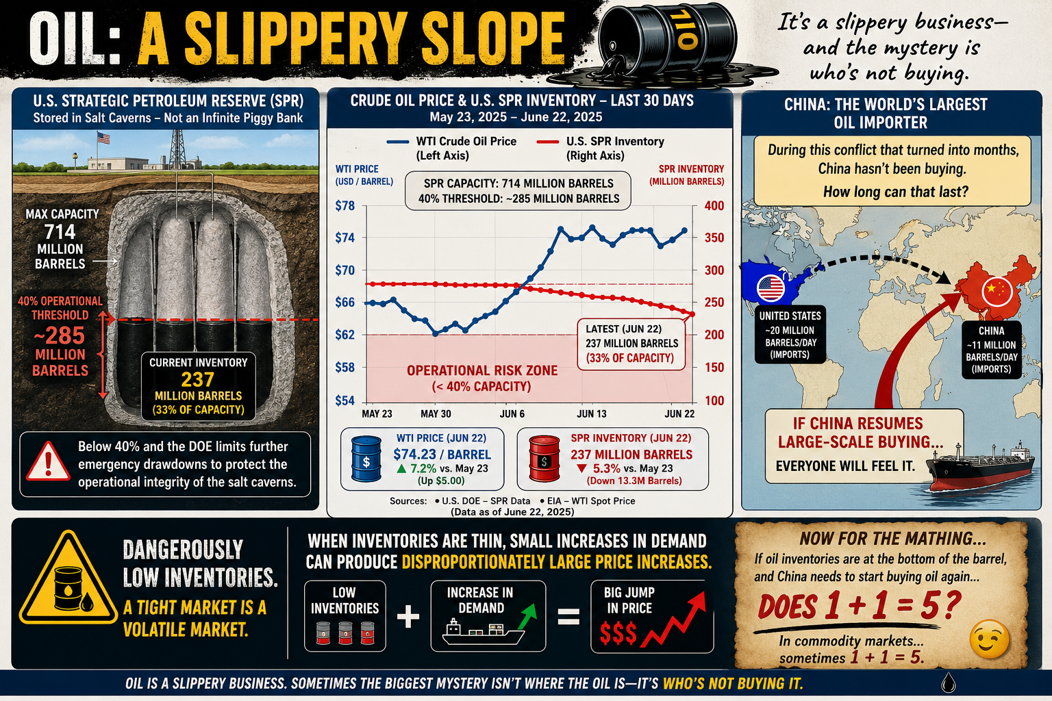
Oil: A Slippery Slope (Literally and Figuratively)

Posted on 2026/07/23 by admin

Oil is one of those subjects that’s surprisingly slippery—both physically and economically. Most people know prices go up and down, but few realize that even storing oil comes with limits.

Take the U.S. Strategic Petroleum Reserve (SPR). It’s often treated like a giant underground gas tank that can be drained and refilled at will. Not quite. The reserve is stored in massive salt caverns, and if inventories fall below roughly 40% of its 714 million-barrel capacity (about 285 million barrels), the Department of Energy limits additional emergency withdrawals. The reason isn’t politics—it’s geology. Keeping enough oil in the caverns helps maintain their long-term operational integrity.

The same basic challenge applies everywhere. Oil storage isn’t as simple as stacking barrels in a warehouse. Tanks, pipelines, and underground caverns all have practical operating limits, and those limits can shape energy policy as much as supply and demand.

Then there’s China.

Despite a conflict that many expected would trigger a buying spree, China has reportedly remained on the sidelines for months rather than aggressively increasing crude purchases. Whether that’s because of existing inventories, weak domestic demand, economic strategy, or expectations of lower future prices is open to debate.

The interesting question isn’t whether China can avoid buying oil today. It’s how long it can continue doing so.

Eventually, inventories run down, demand changes, or market conditions shift. And when one of the world’s largest oil consumers steps back into the market, everyone notices.

Oil has always been a slippery business. Sometimes the biggest mystery isn’t where the oil is—it’s who’s not buying it.

Now for the Math…

If global oil inventories are scraping the bottom of the barrel, and the world’s largest importer suddenly has to start buying again…

…does 1 + 1 = 5?

Not in arithmetic. But in commodity markets, sometimes it feels that way.

When supply is already tight, prices don’t rise in a neat, linear fashion. A relatively small increase in demand can trigger a disproportionately large jump in price as buyers compete for the same limited barrels. Traders see it coming, futures markets react, inventories shrink even faster, and a little bit of demand can snowball into a much bigger price move.

In other words, 1 + 1 doesn’t equal 5 because the math changed—it equals 5 because human behavior did.

Oil markets have always had a nonlinear streak. When inventories are comfortable, an extra million barrels a day barely makes a ripple. But when stocks are running low and spare capacity is scarce, that same million barrels can feel like throwing a match into a room full of gasoline.

That’s why economists watch inventories just as closely as production. Sometimes the most important number isn’t how much oil is being pumped—it’s how much is left in the tank.

Accounting for Climate Responsibility

Posted on 2026/07/23 by admin

by Daniel Brouse

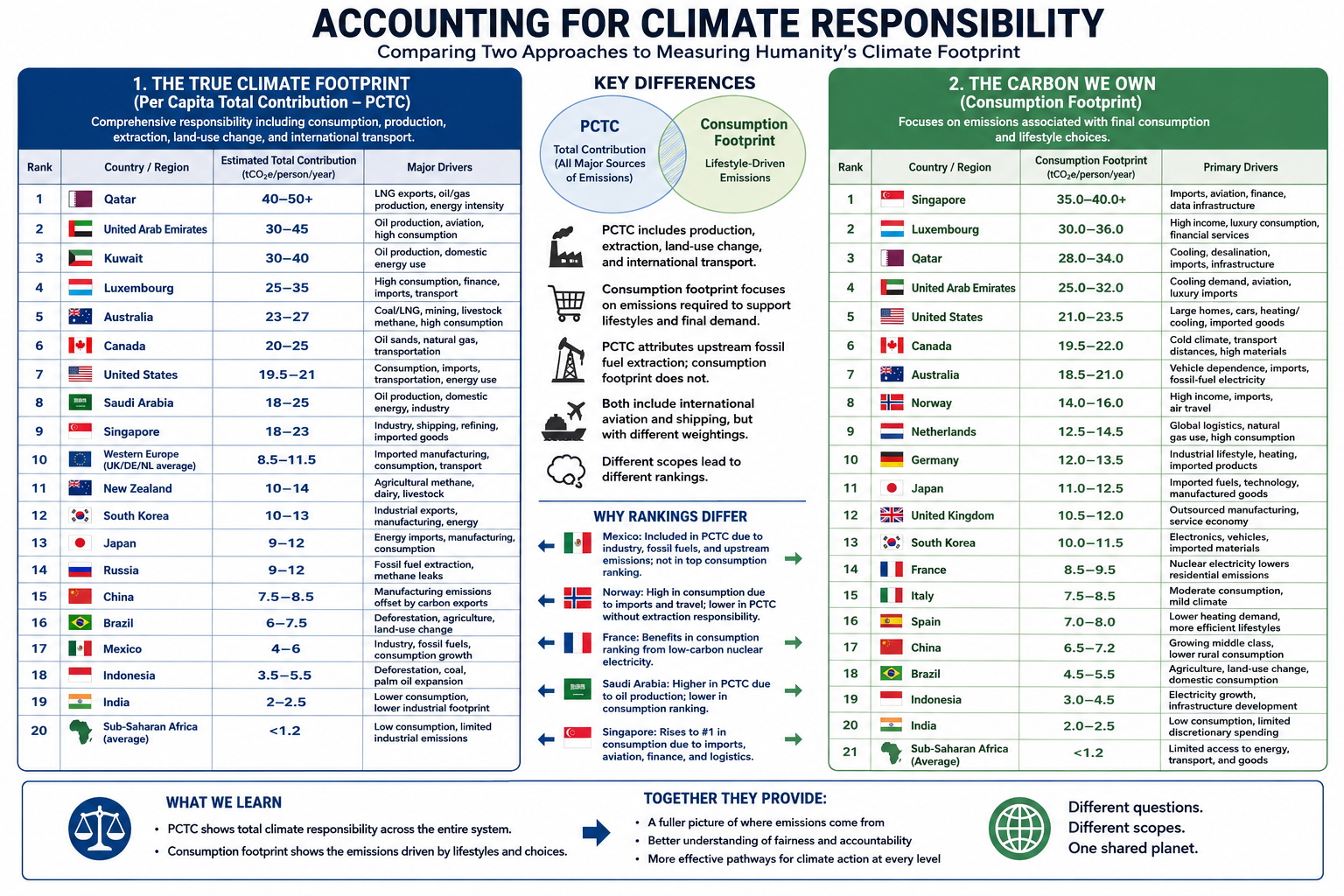
Comparing Two Approaches to Measuring Humanity’s Climate Footprint

Climate responsibility depends on how emissions are assigned. Traditional territorial accounting attributes emissions to the country where they occur, but globalization has made that approach increasingly incomplete. Modern supply chains, international trade, and service-based economies often separate where emissions are produced from who ultimately benefits from them.

To explore this problem from two different perspectives, I developed two complementary accounting frameworks.

The first paper, The True Climate Footprint: Measuring Per Capita Total Contribution Beyond Territorial Emissions, introduces the Per Capita Total Contribution (PCTC) framework. PCTC seeks to estimate an individual’s or nation’s complete climate responsibility by incorporating not only consumption, but also several major sources of emissions that are frequently omitted from conventional carbon accounting.

The True Climate Footprint: Measuring Per Capita Total Contribution

The PCTC framework includes:

Consumption-based emissions
Land-use change and deforestation
Upstream fossil fuel extraction (methane leakage, flaring, and coal mine emissions)
International aviation and maritime shipping
All major greenhouse gases (CO₂, CH₄, N₂O, and others expressed as CO₂-equivalent)
Responsibility associated with fossil fuel production where appropriate

The second paper, The Carbon We Own: Why Consumption Matters More, examines climate responsibility from a different perspective. Rather than estimating total climate contribution, it focuses specifically on the carbon footprint required to support modern lifestyles using a consumption-based accounting approach.

The Carbon We Own: Why Consumption Matters More

This framework emphasizes:

Multi-Regional Input-Output (MRIO) accounting
Direct household energy use
Embedded emissions in imported goods
Public and private services
Lifestyle and purchasing choices

Unlike PCTC, this framework intentionally places less emphasis on fossil fuel extraction and producer responsibility in order to better isolate the climate impacts associated with everyday consumption.

After completing the first paper, I wanted to examine the climate footprint from the perspective of the consumer rather than the entire climate system. The PCTC framework provides a comprehensive measure of total responsibility, but it does not distinguish as clearly between emissions driven by individual lifestyle choices and those associated with resource extraction or national production.

A consumption-based framework highlights decisions that individuals and societies can influence more directly. Choices such as lowering a home’s thermostat, improving insulation, selecting public transportation or electric vehicles instead of internal combustion vehicles, reducing air travel, or purchasing fewer carbon-intensive goods become more visible within the accounting. It also better captures the increasingly important role of service-based economies. While services may appear less energy-intensive than manufacturing, sectors such as healthcare, finance, telecommunications, cloud computing, and artificial intelligence rely on extensive digital infrastructure—including energy-hungry data centers—that can be substantially underrepresented in traditional emissions inventories.

Finally, I wanted a more detailed comparison among developed economies, particularly within Europe. Countries such as Norway and France illustrate why accounting methodology matters. Norway has one of the world’s cleanest domestic electricity systems, powered primarily by hydropower, yet it is also a major exporter of oil and natural gas. France, by contrast, derives much of its electricity from nuclear power, resulting in comparatively low-carbon domestic energy while maintaining a high standard of living. Comparing these countries under both frameworks reveals how different accounting methods assign responsibility and helps illustrate the strengths and limitations of each approach.

Taken together, these two papers do not compete—they answer different questions. Per Capita Total Contribution (PCTC) asks, What is humanity’s full climate responsibility? Consumption-based accounting asks, What emissions are required to sustain the lifestyle of the average resident? Used together, they provide a more complete understanding of climate responsibility than either framework alone.

Conclusion

Although The True Climate Footprint and The Carbon We Own both seek to improve upon traditional territorial emissions accounting, they answer different questions because they are built on different accounting frameworks.

The True Climate Footprint uses the Per Capita Total Contribution (PCTC) framework to estimate an individual’s or nation’s complete contribution to climate change. It extends beyond consumption to include land-use change, upstream fossil fuel extraction, international shipping and aviation, and the full spectrum of greenhouse gases. In some cases, it also attributes responsibility associated with fossil-fuel production, providing a broad measure of humanity’s total climate impact.

By contrast, The Carbon We Own focuses specifically on consumption-based climate responsibility. Using Multi-Regional Input-Output (MRIO) accounting, it assigns emissions to the final consumer by emphasizing direct household energy use, embedded emissions in imported goods, services, and lifestyle choices. It intentionally deemphasizes extraction and producer responsibility in order to better represent the carbon footprint required to sustain modern patterns of consumption.

Because these frameworks measure different aspects of climate responsibility, their rankings are not expected to be identical.

Mexico provides a useful illustration. Under the PCTC framework, Mexico’s estimated footprint includes domestic industry, fossil fuel production, growing consumption, and upstream emissions, resulting in an estimated contribution of approximately 4–6 tonnes of CO₂-equivalent per person per year. In the consumption-based analysis, however, Mexico does not appear among the highest-ranking countries because the focus is limited to end-user consumption, and the published rankings emphasize the world’s largest per-capita consumption footprints.

Similar differences appear elsewhere. Norway’s position changes substantially because one framework incorporates the climate responsibility associated with fossil fuel production, while the other emphasizes domestic consumption. France benefits in the consumption-based analysis because its low-carbon nuclear electricity reduces household emissions despite maintaining a high standard of living. Saudi Arabia ranks differently depending on whether responsibility is assigned to oil production or to energy consumption. Singapore rises dramatically under consumption accounting because imported goods, international aviation, finance, logistics, and digital infrastructure contribute heavily to its consumption footprint despite relatively limited domestic manufacturing.

These examples demonstrate that accounting methodology influences how climate responsibility is distributed. Production-based, consumption-based, and total-contribution frameworks each illuminate different dimensions of the global climate system.

Rather than viewing these approaches as competing methodologies, they should be regarded as complementary analytical tools. The Per Capita Total Contribution (PCTC) framework asks, What is a nation’s or individual’s total contribution to climate change? The consumption-based framework asks, What emissions are required to sustain the average resident’s lifestyle? Together, they provide a more complete understanding of climate responsibility than either approach can achieve alone, revealing both the systemic impacts of resource production and the powerful role of consumer demand in shaping the global climate.

The Carbon We Own: Why Consumption Matters More

Posted on 2026/07/222026/07/23 by admin

by Daniel Brouse

For decades, climate responsibility has often been measured by where fossil fuels are extracted or where products are manufactured. While useful for tracking national emissions, this production-based approach can misrepresent who ultimately drives demand.

A consumption-based accounting approach shifts the focus to the end user. Instead of assigning emissions to the country where a product is made, it attributes emissions to the people and businesses that ultimately consume the energy, goods, and services.

Under this framework, every kilowatt-hour of electricity, every heating bill, every medical service, and every consumer product is assigned to its final destination.

For example, if a smartphone is manufactured in Asia using electricity generated from coal and then shipped across the Pacific to a consumer in Los Angeles, the emissions associated with mining, manufacturing, transportation, and delivery are attributed to the American consumer—not the manufacturing country.

This approach provides a more accurate picture of the carbon footprint associated with modern lifestyles.

How Consumption-Based Carbon Accounting Works

Most consumption analyses rely on Multi-Regional Input-Output (MRIO) economic models, which trace emissions through global supply chains before assigning them to final consumers.

Individual carbon footprints are generally divided into three major categories:

1. Direct Household Energy

Emissions from energy used directly by households, including:

Home heating and cooling
Residential electricity
Personal vehicle fuel
Digital activities such as internet usage and streaming services

2. Embedded Goods

Emissions generated while producing and transporting purchased products, including:

Electronics
Vehicles
Furniture
Clothing
Building materials
Household appliances

These emissions often occur in countries far from the final consumer.

3. Services

Many of the largest emissions in developed economies come not from physical products but from services, including:

Healthcare
Commercial aviation
Banking and finance
Cloud computing
Water and wastewater treatment
Telecommunications

In the United States alone, healthcare contributes roughly 1.6 tonnes of CO₂-equivalent emissions per person each year, illustrating how service-based economies can generate substantial carbon footprints even as heavy industry declines.

Major Findings from Global Consumption Accounting

The Rise of Service Economies

In wealthy economies such as Singapore, Luxembourg, and several Western European countries, manufacturing represents only a small portion of domestic emissions.

Instead, much of their climate impact comes from:

Commercial aviation
Financial systems
Cloud computing
Global logistics
Luxury consumption
High levels of imported goods

As economies become increasingly service-oriented, carbon emissions become embedded in complex international supply chains rather than local smokestacks.

Geography Still Matters

Climate strongly influences direct household energy use.

Countries with long, cold winters or extremely hot summers require substantially more energy for climate control.

For example:

Canada and the United States consume large amounts of energy for winter heating and summer air conditioning, particularly because of larger average home sizes.
Australia records comparatively higher emissions from agriculture, mining, and infrastructure development than from residential heating.

Local climate remains an important contributor even after imported goods are included.

China’s Manufacturing Versus Consumption

China illustrates one of the largest differences between production-based and consumption-based accounting.

Because China manufactures enormous quantities of products for export, its territorial emissions are among the highest in the world.

However, when emissions are allocated to the people who ultimately purchase those products, China’s domestic per-capita consumption footprint is estimated at roughly 6.8 tonnes of CO₂-equivalent per year.

This highlights the distinction between:

Production emissions (where goods are made)
Consumption emissions (who ultimately benefits from those goods)

Many products manufactured in China are consumed in North America and Europe, meaning a significant share of manufacturing emissions is driven by foreign demand.

Consumption Footprints Across Europe

Norway: Clean Electricity, High Consumption

Estimated consumption footprint: 14.8 tonnes CO₂e per person

Norway’s electricity is more than 85% hydropower, giving it one of the cleanest electrical grids in the world.

Yet Norwegians have high purchasing power and consume large quantities of imported goods, including:

Electric vehicles
Consumer electronics
Luxury goods
Imported foods

Norway also has one of the world’s highest rates of air travel per capita, increasing its service-sector emissions.

The result is a consumption footprint considerably larger than its territorial emissions suggest.

United Kingdom: Outsourcing Manufacturing

Estimated consumption footprint: 11.2 tonnes CO₂e per person

The United Kingdom has significantly reduced domestic production emissions by retiring coal-fired power plants and expanding renewable electricity.

However, much of the country’s manufacturing has shifted overseas.

The UK imports large quantities of:

Electronics
Machinery
Clothing
Construction materials

Consequently, much of its carbon footprint exists outside its borders, while domestic emissions increasingly come from finance, digital infrastructure, commercial services, and transportation.

France: The Nuclear Advantage

Estimated consumption footprint: 9.2 tonnes CO₂e per person

France demonstrates how a low-carbon electricity system can substantially reduce consumption emissions.

French households enjoy living standards comparable to neighboring Western European countries, yet much of their residential electricity, rail transportation, and heating is supplied by nuclear energy.

As a result, France’s direct household energy emissions are estimated to be roughly 30% lower than those of many neighboring countries with similar consumption patterns.

China Compared with Western Europe

When emissions are assigned to consumers rather than producers, an average citizen in countries such as Germany or the United Kingdom is responsible for nearly twice the carbon footprint of the average Chinese citizen.

Although China’s middle class continues to grow and domestic consumption is increasing, much of the country’s industrial output still serves international markets.

This comparison illustrates a key insight of consumption-based accounting:

A nation’s production does not necessarily reflect the climate impact of its residents’ lifestyles.

A Different Way to Think About Climate Responsibility

Consumption-based accounting reframes climate responsibility by asking a simple question:

Who ultimately benefits from the energy and resources consumed?

Rather than focusing solely on where emissions occur, this approach follows products and services through global supply chains to their final users.

For affluent economies that import large volumes of manufactured goods while exporting much of their industrial production, consumption-based accounting often reveals substantially higher per-capita climate footprints than traditional territorial inventories.

Viewed through this lens, lifestyle choices, purchasing power, housing, transportation, travel, healthcare, digital services, and overall consumption patterns become the primary drivers of individual climate responsibility.

Ultimately, the atmosphere responds to total emissions, regardless of where they occur. Consumption-based accounting provides a complementary perspective to traditional production-based inventories by connecting those emissions to the people and economies whose demand created them.

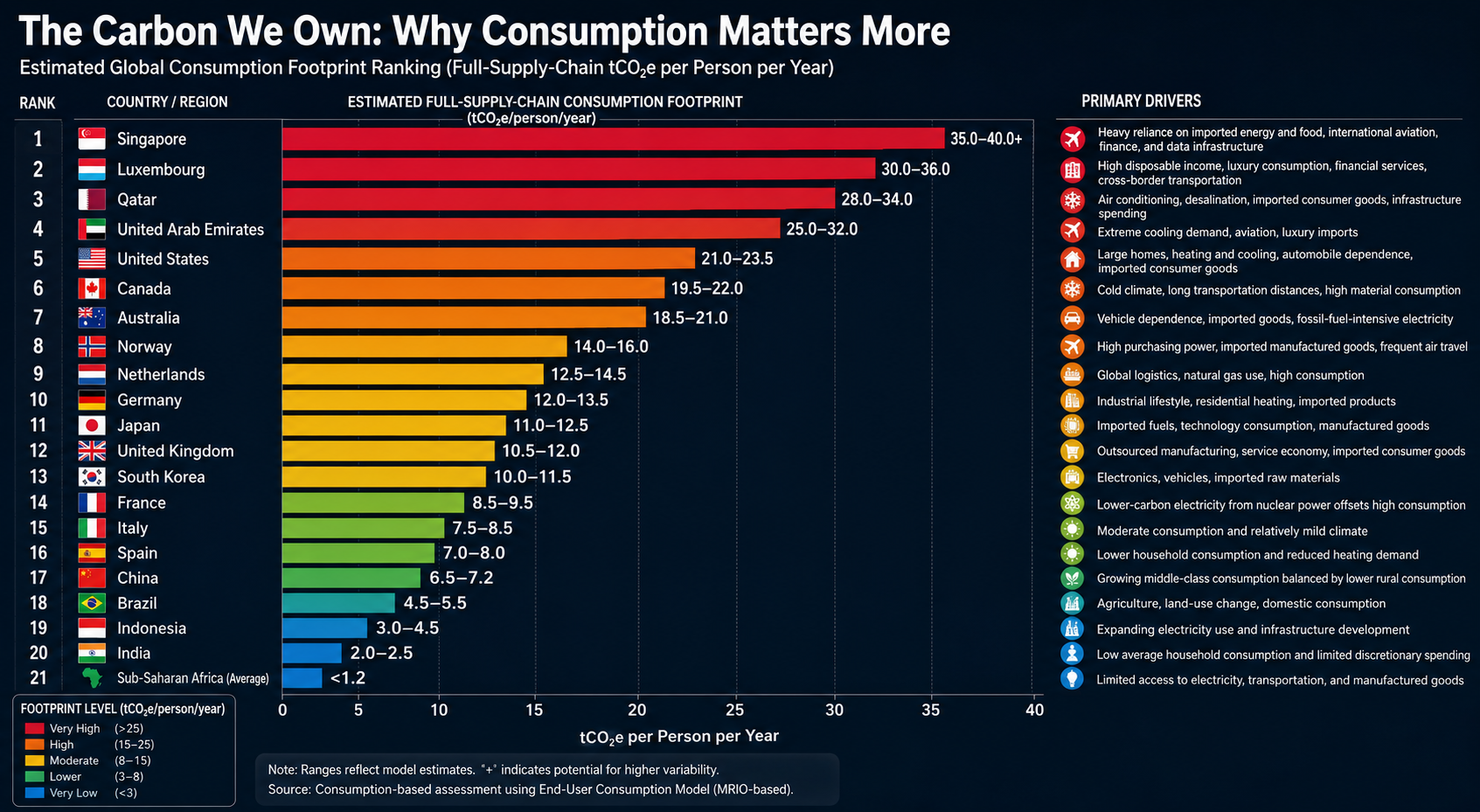
Global Consumption Footprint Rankings

Traditional emissions inventories assign carbon pollution to the country where fossil fuels are extracted or products are manufactured. A consumption-based accounting approach instead assigns those emissions to the people and economies that ultimately consume the goods and services.

The rankings below are based on an End-User Consumption Model, which allocates the full upstream supply-chain emissions—including raw material extraction, manufacturing, international transportation, agricultural land-use change, and other embedded emissions—to the final purchaser.

Rather than measuring where emissions occur, this framework estimates the carbon footprint required to sustain the average lifestyle of a country’s residents. It reflects direct household energy use, consumption of imported goods, transportation, public infrastructure, and carbon-intensive services.

Estimated Global Consumption Footprint Ranking

Rank	Country / Region	Estimated Full-Supply-Chain Consumption Footprint (tCO₂e/person/year)	Primary Drivers
1	🇸🇬 Singapore	35.0–40.0+	Heavy reliance on imported energy and food, international aviation, finance, and data infrastructure
2	🇱🇺 Luxembourg	30.0–36.0	High disposable income, luxury consumption, financial services, cross-border transportation
3	🇶🇦 Qatar	28.0–34.0	Air conditioning, desalination, imported consumer goods, infrastructure spending
4	🇦🇪 United Arab Emirates	25.0–32.0	Extreme cooling demand, aviation, luxury imports
5	🇺🇸 United States	21.0–23.5	Large homes, heating and cooling, automobile dependence, imported consumer goods
6	🇨🇦 Canada	19.5–22.0	Cold climate, long transportation distances, high material consumption
7	🇦🇺 Australia	18.5–21.0	Vehicle dependence, imported goods, fossil-fuel-intensive electricity
8	🇳🇴 Norway	14.0–16.0	High purchasing power, imported manufactured goods, frequent air travel
9	🇳🇱 Netherlands	12.5–14.5	Global logistics, natural gas use, high consumption
10	🇩🇪 Germany	12.0–13.5	Industrial lifestyle, residential heating, imported products
11	🇯🇵 Japan	11.0–12.5	Imported fuels, technology consumption, manufactured goods
12	🇬🇧 United Kingdom	10.5–12.0	Outsourced manufacturing, service economy, imported consumer goods
13	🇰🇷 South Korea	10.0–11.5	Electronics, vehicles, imported raw materials
14	🇫🇷 France	8.5–9.5	Lower-carbon electricity from nuclear power offsets high consumption
15	🇮🇹 Italy	7.5–8.5	Moderate consumption and relatively mild climate
16	🇪🇸 Spain	7.0–8.0	Lower household consumption and reduced heating demand
17	🇨🇳 China	6.5–7.2	Growing middle-class consumption balanced by lower rural consumption
18	🇧🇷 Brazil	4.5–5.5	Agriculture, land-use change, domestic consumption
19	🇮🇩 Indonesia	3.0–4.5	Expanding electricity use and infrastructure development
20	🇮🇳 India	2.0–2.5	Low average household consumption and limited discretionary spending
21	Sub-Saharan Africa (Average)	<1.2	Limited access to electricity, transportation, and manufactured goods

Key Patterns

Small, Wealthy Nations Have the Largest Per-Capita Footprints

Singapore and Luxembourg rank highest despite having relatively little domestic heavy industry. Their residents consume large quantities of imported goods and services, while extensive international transportation, finance, aviation, and digital infrastructure contribute substantial embedded emissions.

High-Income, Car-Oriented Economies Form the Next Tier

The United States, Canada, and Australia consistently rank among the world’s largest per-capita consumers. Large homes, automobile-dependent communities, extensive heating or cooling needs, and high levels of discretionary consumption combine to produce substantial lifestyle-related emissions.

Low-Carbon Electricity Helps—but Doesn’t Eliminate Consumption Emissions

Countries such as France and Norway demonstrate that cleaner electricity significantly lowers household energy emissions. However, imported goods, international travel, and service-sector activities remain important contributors to their overall consumption footprints.

Manufacturing Countries Are Not Necessarily the Largest Consumers

China’s production-based emissions are among the highest globally because it manufactures goods for international markets. Under a consumption-based framework, however, the average Chinese citizen’s lifestyle footprint remains considerably lower than that of residents in many affluent Western countries.

Consumption Capacity Is the Strongest Predictor

Perhaps the clearest finding is the enormous gap between affluent economies and developing regions. Average per-capita consumption in Sub-Saharan Africa remains a small fraction of that in the world’s wealthiest nations, reflecting differences in income, energy access, transportation, housing, and consumer purchasing power.

This comparison underscores a central conclusion of consumption-based accounting: the carbon footprint of an individual is driven primarily by the scale and complexity of the lifestyle they support, rather than the geographic location where the associated emissions physically occur.

The True Climate Footprint: Measuring Per Capita Total Contribution

Posted on 2026/07/222026/07/22 by admin

by Daniel Brouse

Why Traditional Carbon Accounting Underestimates Responsibility

Climate responsibility is often measured using territorial emissions: the greenhouse gases released within a country’s borders. While useful, this approach does not capture the full climate footprint of modern economies because it ignores global supply chains, outsourced manufacturing, land-use change, and upstream fossil fuel emissions.

A more complete measure requires calculating Per Capita Total Contribution—a footprint-based accounting system that assigns responsibility based on the full lifecycle of consumption and environmental impact.

This approach combines:

Consumption-based emissions accounting — tracking emissions embedded in imported goods and services.
Land Use Change (LUC) — including deforestation, agricultural expansion, and ecosystem conversion.
Upstream fossil fuel emissions — including methane leaks, flaring, and coal mine emissions.
International transportation — including aviation and shipping.
All greenhouse gases — not just carbon dioxide, but methane, nitrous oxide, and other climate pollutants.

Using this broader framework, humanity’s total annual climate footprint rises to approximately 53.5 billion tonnes of CO₂-equivalent (CO₂e), or about 6.6 tonnes of CO₂e per person globally.

However, once these factors are included, the global map of climate responsibility changes dramatically.

1. The Hidden Carbon Footprint of Global Trade

Outsourced Emissions: When Consumption Drives Pollution Elsewhere

Traditional accounting assigns emissions to the country where goods are produced. This creates a major distortion in a globalized economy.

Consumption-based accounting reverses this by:

Subtracting emissions from exports.
Adding emissions embedded in imports.
Assigning responsibility to the final consumer.

This reveals a significant shift:

Western Consumption Footprints Expand

Many wealthy nations have reduced domestic industrial emissions partly by moving manufacturing overseas. Electronics, clothing, machinery, and other consumer products may be manufactured in China or Southeast Asia, but much of the demand originates in North America and Europe.

The emissions occur in the producing country, but the consumption benefit occurs elsewhere.

Carbon Exporters vs. Carbon Importers

Under territorial accounting:

Manufacturing nations appear more responsible.
Consumer nations appear cleaner.

Under footprint accounting:

Major consumer economies become large net importers of carbon emissions.
Manufacturing hubs become net exporters of embedded carbon.

2. The Missing Climate Cost of Land Use Change

Deforestation and land conversion contribute roughly 10% of global greenhouse gas emissions.

However, these emissions are rarely assigned to the ultimate consumers driving demand.

A complete accounting system tracks:

Beef production linked to Amazon clearing.
Soy expansion replacing forests.
Palm oil plantations.
Timber extraction.
Agricultural conversion.

Consumer-Driven Deforestation Footprints

Some nations experience a substantial increase in their climate footprint when imported commodities are included.

Examples:

Wealthy food-importing nations may carry a larger footprint because their consumption drives land clearing elsewhere.
Countries such as Brazil and Indonesia receive major additions from domestic land-use change before those emissions are redistributed through trade.

3. Fossil Fuel Extraction: Counting the Full Climate Cost

Burning fossil fuels is only part of their climate impact.

A complete footprint must include emissions from extraction:

Methane leakage from oil and gas production.
Coal mine methane releases.
Flaring.
Venting during production and transport.

Methane is especially important because it is approximately 30 times more powerful than carbon dioxide over a 100-year period.

Territorial accounting can distort responsibility:

Fossil fuel exporters may appear responsible for extraction emissions occurring within their borders.
Consumer nations benefit from the energy but avoid the associated extraction footprint.

A true accounting system assigns these emissions across the entire fossil fuel supply chain, including the countries ultimately consuming the energy.

The Recalculated Climate Responsibility Landscape

Country / Region	Standard Territorial CO₂ (Fossil Fuels Only)	Estimated Total Contribution (All GHGs + Trade + Land Use + Transport)	Primary Driver of Change
United States	~14.9 tonnes/person	~19.5–21.0 tonnes/person	High consumption, imported manufacturing, carbon-intensive lifestyles
Western Europe	~4.5–7.0 tonnes/person	~8.5–11.5 tonnes/person	Outsourced manufacturing and imported goods
China	~8.0 tonnes/person	~7.5–8.5 tonnes/person	Large manufacturing exporter offsets domestic emissions
Brazil	~2.3 tonnes/person	~6.0–7.5 tonnes/person	Deforestation and agricultural land conversion
India	~2.0 tonnes/person	~2.2 tonnes/person	Lower consumption footprint
Sub-Saharan Africa	<1.0 tonnes/person	<1.2 tonnes/person	Low consumption and limited industrial emissions

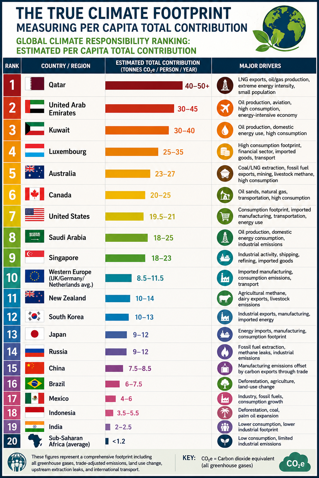
Global Climate Responsibility Ranking: Estimated Per Capita Total Contribution

Rank	Country / Region	Estimated Total Contribution (Tonnes CO₂e/person/year)	Major Drivers
1	Qatar	40–50+	LNG exports, oil/gas production, extreme energy intensity, small population
2	United Arab Emirates	30–45	Oil production, aviation, high consumption, energy-intensive economy
3	Kuwait	30–40	Oil production, domestic energy use, high consumption
4	Luxembourg	25–35	High consumption footprint, financial sector, imported goods, transport
5	Australia	23–27	Coal/LNG extraction, fossil fuel exports, mining, livestock methane, high consumption
6	Canada	20–25	Oil sands, natural gas, transportation, high consumption
7	United States	19.5–21	Consumption footprint, imported manufacturing, transportation, energy use
8	Saudi Arabia	18–25	Oil production, domestic energy consumption, industrial emissions
9	Singapore	18–23	Industrial activity, shipping, refining, imported goods
10	Western Europe (UK/Germany/Netherlands average)	8.5–11.5	Imported manufacturing, consumption emissions, transport
11	New Zealand	10–14	Agricultural methane, dairy exports, livestock emissions
12	South Korea	10–13	Industrial exports, manufacturing, imported energy
13	Japan	9–12	Energy imports, manufacturing, consumption footprint
14	Russia	9–12	Fossil fuel extraction, methane leaks, industrial emissions
15	China	7.5–8.5	Manufacturing emissions offset by carbon exports through trade
16	Brazil	6–7.5	Deforestation, agriculture, land-use change
17	Mexico	4–6	Industry, fossil fuels, consumption growth
18	Indonesia	3.5–5.5	Deforestation, coal, palm oil expansion
19	India	2–2.5	Lower consumption, lower industrial footprint
20	Sub-Saharan Africa (average)	<1.2	Low consumption, limited industrial emissions

The Real Climate Equation: Consumption × Population × Technology

The climate challenge is often framed as a population problem. However, the dominant driver of emissions is not simply the number of people on Earth—it is the per capita intensity of resource consumption and pollution.

A more accurate equation is: $\textbf{Total Climate Impact} = \textbf{Population} \times \textbf{Per Capita Consumption} \times \textbf{Carbon Intensity}$ Total Climate Impact=Population×Per Capita Consumption×Carbon Intensity

Population matters, but consumption patterns and technology determine the magnitude of environmental impact.

A world with billions more people using efficient, low-carbon systems could have a smaller footprint than a smaller population consuming resources at current high-intensity levels.

Toward a Fairer Climate Accounting System

Territorial emissions remain useful for tracking national inventories, but they do not fully capture responsibility in a globalized economy.

A true Per Capita Total Contribution framework recognizes that climate change is driven by:

Who consumes resources.
Who benefits from production.
Who drives land conversion.
Who extracts and burns fossil fuels.
Who has the technological and economic capacity to reduce emissions.

The future of climate accountability depends on moving beyond borders and measuring the complete human footprint on Earth.

Conclusion

The climate conversation has focused on the wrong number.

The problem isn’t simply how many people live on Earth.

It’s how each of us lives.

The average person on the planet is responsible for about 6.6 tonnes of CO₂e per year, but the differences between countries are staggering. Some affluent societies generate 20–50+ tonnes per person, while much of the developing world contributes less than 2 tonnes.

That’s why climate responsibility is better measured by per capita total contribution—including consumption, outsourced manufacturing, deforestation, fossil fuel extraction, agriculture, and transportation—not just emissions produced within national borders.

A child born into a high-consumption lifestyle can have a climate footprint many times larger than several people living in low-consumption economies.

The challenge is not humanity itself.

The challenge is how we consume, how we produce, and how much we extract from the planet.

Changing lifestyles, improving efficiency, and transitioning to cleaner energy can reduce our impact without reducing our humanity.

The future depends less on the number of people—and more on the choices each of us makes.

2026 Climate Disasters: A Year of Escalating Heat, Floods, Storms, and Climate Amplification

Posted on 2026/07/222026/07/22 by admin

by Daniel Brouse

A Global Climate System Under Increasing Stress

The most destructive climate disasters of 2026 reveal a rapidly changing pattern: extreme events are becoming more intense, more widespread, and increasingly interconnected.

From deadly heatwaves across Europe and South Asia to catastrophic flooding and severe storms across the United States, this year’s disasters demonstrate how human-caused warming is amplifying natural climate variability.

Scientific attribution studies from organizations such as World Weather Attribution (WWA) have repeatedly shown that greenhouse gas emissions are increasing the severity, duration, and likelihood of many modern climate extremes. Climate change is not replacing natural weather patterns—it is shifting the baseline conditions in which those patterns occur, turning historically rare events into recurring hazards.

1. Global Heatwaves and Heat Domes — The Deadliest Climate Hazard of 2026

Extreme heat has emerged as the defining climate disaster of the year, affecting billions of people across South Asia, Europe, the Middle East, and North America.

South Asia: Record-Breaking Pre-Monsoon Heat

India and Pakistan experienced a prolonged pre-monsoon heatwave, with temperatures repeatedly exceeding 46°C (115°F) in multiple cities.

The extreme heat disrupted agriculture, increased energy demand, threatened outdoor workers, and placed millions of vulnerable people at risk.

Climate Connection:
World Weather Attribution researchers concluded that human-caused warming significantly intensified the event, making such prolonged extreme heat far more likely than under historical climate conditions.

Europe: Over 10,000 Excess Deaths from Extreme Heat

Europe experienced one of the most severe heat disasters in modern history as persistent heatwaves pushed temperatures 5–12°C above average in some regions.

France, Spain, the United Kingdom, and other European nations experienced record-breaking temperatures, widespread drought stress, increased wildfire danger, and severe impacts on public health.

The heat contributed to more than 10,000 excess deaths, with older adults and people with underlying health vulnerabilities experiencing the greatest risks.

These deaths highlight the growing recognition that extreme heat is one of the deadliest consequences of climate change, often exceeding the immediate fatalities associated with storms and floods.

Climate Connection:
Attribution studies have concluded that human-caused climate change substantially increased the intensity and probability of these European heat extremes by raising the global temperature baseline.

The Hajj Heat Disaster: Climate Risks in a Warmer World

In Mecca, Saudi Arabia, extreme heat during the Hajj pilgrimage created dangerous conditions for millions of participants.

The combination of intense solar exposure, high humidity, and prolonged outdoor activity pushed temperatures beyond historically safe thresholds, producing hundreds of heat-related illnesses and significant loss of life.

Climate Connection:
Fossil fuel emissions have expanded the duration and severity of dangerous heat conditions in the region, increasing risks for large outdoor gatherings.

2. The Emerging Super El Niño: A Climate Amplifier

The extreme weather of 2026 is occurring alongside a strengthening El Niño event in the tropical Pacific.

El Niño is a natural climate cycle that periodically transfers large amounts of ocean heat into the atmosphere. However, it is now occurring on top of record global ocean temperatures driven by greenhouse gas emissions.

This creates a climate multiplier effect, increasing the likelihood of:

Record-breaking temperatures
Extreme rainfall events
Flash flooding
Agricultural disruption
Expanding drought conditions

The interaction between natural variability and human-caused warming is producing a more unstable and energetic climate system.

Major U.S. Climate Disasters of 2026

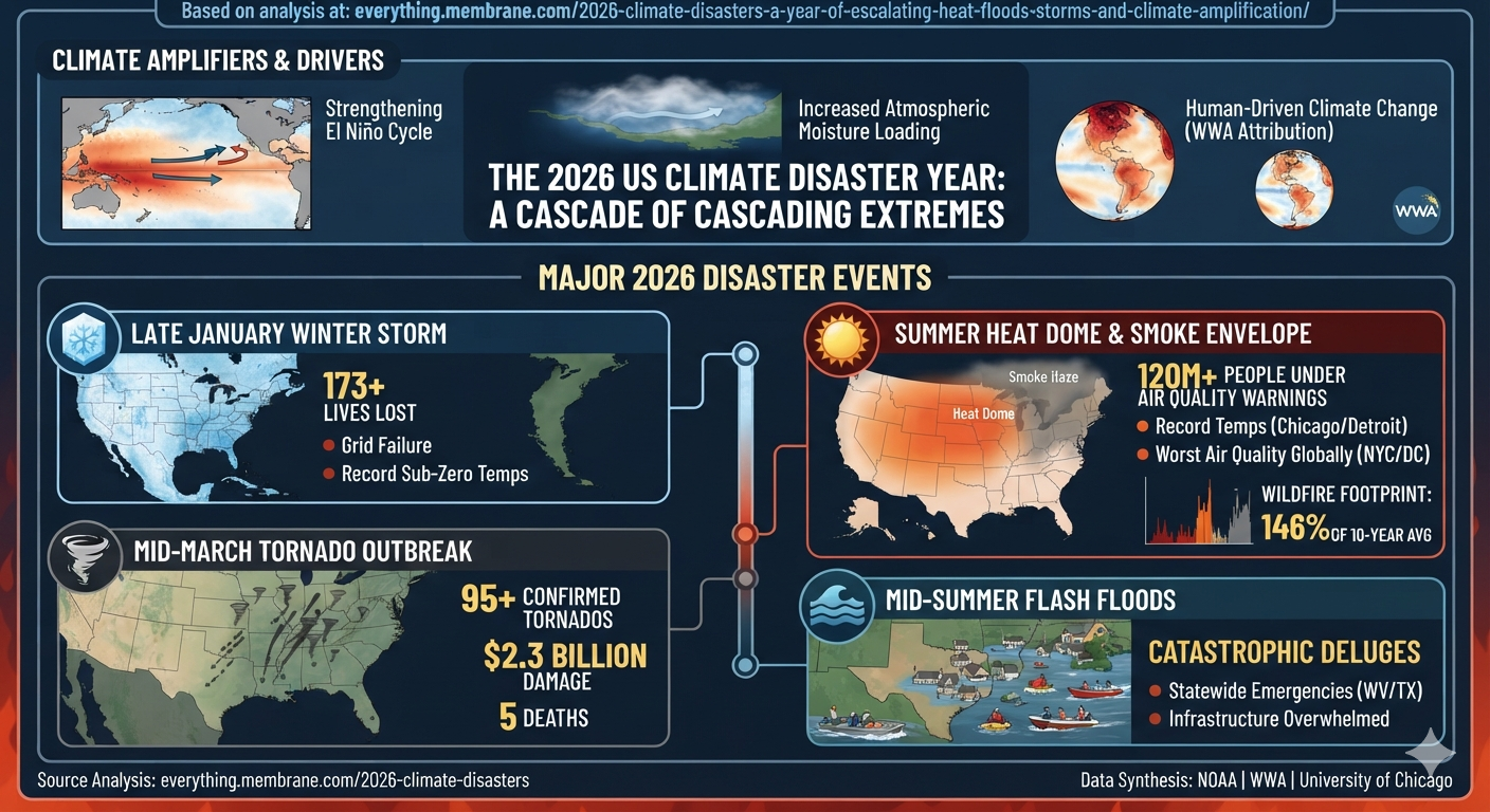
1. Summer Heat Dome and Wildfire Smoke Envelope — Largest Human Exposure

The most widespread U.S. climate disaster of the year was a massive heat dome combined with wildfire smoke spreading across the continent.

More than 120 million Americans from Minnesota to Massachusetts experienced heat alerts and hazardous air quality conditions.

Major metropolitan areas including Chicago, Detroit, New York, and Washington, D.C., experienced some of the worst air quality conditions in the world as smoke from Canadian wildfires moved southward.

Climate Connection:
Hotter and drier conditions have expanded wildfire activity, with North American wildfire acreage reaching approximately 146% of the 10-year average. Climate change is increasing the likelihood of persistent heat domes, drought conditions, and larger wildfire seasons.

2. January North American Winter Storm — Highest Early-Year Death Toll

A massive winter storm swept across the United States and Atlantic Canada, producing extreme cold, freezing temperatures, ice accumulation, and infrastructure failures.

The storm caused more than 173 deaths, making it one of the deadliest weather events of the year.

Climate Connection:
Although winter storms remain natural phenomena, warmer oceans and a warmer atmosphere allow storms to carry more moisture, increasing the potential for heavier precipitation, extreme snowfall, and more damaging freeze events.

3. Central and Southeastern Tornado Outbreak — Largest Severe Storm Damage

A three-day severe weather outbreak in March produced more than 95 confirmed tornadoes, causing approximately $2.3 billion in damage.

The storms moved from Illinois into Mississippi, Alabama, and Georgia, producing destructive tornadoes, damaging winds, and widespread infrastructure impacts.

Climate Connection:
A warmer atmosphere contains more heat and moisture, increasing atmospheric instability and creating conditions favorable for more intense severe thunderstorms.

4. Mid-Summer Flash Flood Disasters — The Fastest Escalating Threat

Extreme rainfall events produced catastrophic flash flooding across parts of Texas Hill Country, West Virginia, and the Ohio Valley.

Communities experienced emergency declarations, water rescues, landslides, infrastructure failures, and overwhelmed emergency systems.

Climate Connection:
Because the atmosphere holds approximately 7% more moisture for every 1°C of warming, climate change is increasing the potential for sudden, extreme rainfall events that overwhelm drainage systems and communities.

2026 Climate Disaster Overview

Disaster Category	Key 2026 Indicator	Major Impact Areas
Extreme Heat	Record-breaking heatwaves and >10,000 European excess deaths	Europe, South Asia, Middle East, North America
Wildfires	146% of 10-year average acreage burned	Western U.S., Canada, Northeast smoke corridor
Severe Storms	$2.3 billion tornado outbreak	Illinois, Mississippi, Alabama, Georgia
Flash Flooding	Multiple emergency declarations	Texas Hill Country, West Virginia, Ohio Valley
Winter Storms	173+ fatalities	United States and Atlantic Canada

A New Era of Compound Climate Disasters

The defining feature of 2026 is not simply that individual disasters are becoming stronger—it is that climate extremes are increasingly interacting.

Heat intensifies drought.
Drought fuels wildfires.
Wildfires spread smoke across continents.
Warmer oceans energize storms.
A warmer atmosphere produces heavier rainfall.

These cascading interactions represent a transition from isolated weather events to a more interconnected climate risk system.

The challenge of the coming decades will not only be adapting to a warmer planet, but managing a climate system where multiple extreme events increasingly occur together, amplify one another, and create cascading impacts across societies and ecosystems.

From Linear Warming to Cascading Climate Dynamics: The Evolution Toward a Nonlinear Earth System Framework

Posted on 2026/07/222026/07/22 by admin

By Daniel Brouse and Sidd Mukherjee

For decades, climate change has been communicated primarily through a relatively simple causal framework: increasing greenhouse gas concentrations drive global warming, which then increases the frequency, intensity, and duration of climate impacts. This linear model has been extraordinarily successful in explaining the fundamental physics of anthropogenic climate change.

However, Earth’s climate system is not a simple linear machine. It is a complex adaptive system composed of interacting components—including the atmosphere, oceans, cryosphere, biosphere, and human systems—that continuously exchange energy, matter, and information. As these interactions strengthen, the climate system can exhibit behaviors that cannot be fully explained by examining individual components in isolation.

In the 1990s, together with laboratory partner Sidd Mukherjee, we began developing the Nonlinear Acceleration Hypothesis (NAH), a framework proposing that climate change evolves through increasingly interconnected feedback networks. The hypothesis suggests that as climate subsystems become more tightly coupled, disturbances can propagate across multiple pathways, accelerating the rate of environmental change and increasing the probability of compound and cascading climate events.

At the center of this framework is the concept of the Domino Effect, or Cascading Climate Dynamics. In this view, climate-driven events are not isolated occurrences but interacting processes in which one disturbance alters the conditions that influence subsequent events.

For example:

Rising temperatures → increased atmospheric moisture → stronger precipitation extremes → flooding → ecosystem disruption → economic impacts → societal stress

Similarly:

Arctic warming → permafrost thaw → greenhouse gas release → additional warming → further ice loss

These cascading interactions create reinforcing feedback loops that can reshape the trajectory of the entire Earth system.

Climate State-Space: Mapping Earth’s Changing Trajectory

The concept of climate state-space modeling provides a mathematical framework for understanding these complex transitions. Rather than describing climate change through a single variable such as global average temperature, state-space analysis represents the Earth system as a multidimensional landscape containing interacting variables such as:

Ocean heat content
Sea level rise
Atmospheric water vapor
Marine heatwaves
Ice-sheet stability
Ecosystem resilience
Extreme weather frequency

Each combination of these variables represents a possible climate state. As greenhouse forcing increases and feedback mechanisms intensify, Earth does not simply become warmer—it migrates through climate state-space toward increasingly unfamiliar regions characterized by new combinations of environmental conditions.

This perspective explains why modern climate extremes are increasingly difficult to categorize using historical experience alone. The challenge is not only that individual variables are changing, but that the relationships among variables are also evolving.

Extreme Event Attribution: The Missing Link Supporting a Nonlinear Climate Framework

For many years, climate science was able to establish the broad relationship between rising greenhouse gas concentrations and a warming planet, but scientists faced a significant challenge: determining the extent to which human-caused climate change contributed to specific individual extreme events.

That limitation has now been substantially reduced. Recent advances in extreme event attribution science, including the landmark work summarized by the National Academies of Sciences, Engineering, and Medicine (NASEM), have demonstrated that researchers can rigorously evaluate the human contribution to individual climate extremes, including heatwaves, heavy precipitation events, droughts, and other high-impact phenomena.

This scientific advancement represents more than an improvement in attribution methods—it provides critical observational support for the transition from a linear climate model toward a nonlinear Earth system framework.

The ability to attribute individual events to anthropogenic forcing confirms that climate change is not merely a gradual shift in global averages. Human influence is now detectable within specific components of the climate system and within the extreme events that emerge from their interactions.

This directly aligns with the central premise of the Nonlinear Acceleration Hypothesis (NAH): that climate change increasingly operates through interconnected feedback networks where individual disturbances can amplify, propagate, and interact across multiple Earth system components.

The scientific question is therefore evolving from:

“Is human activity causing climate change and increasing extreme events?”

to:

“How do human-driven changes alter the probability, intensity, timing, and interaction of cascading climate events across the Earth system?”

NASEM’s validation of extreme event attribution establishes an important foundation for this next phase of climate science. If human influence can now be detected within individual extreme events, then the logical next step is understanding how these events connect through feedback loops and contribute to broader system-level transitions.

The emerging scientific picture is of a coupled planetary system in which the atmosphere, oceans, cryosphere, biosphere, and human societies are not independent components but interacting elements of a dynamic network.

The future of climate research must therefore expand beyond measuring warming alone and toward understanding climate system acceleration, state-space migration, and cascading dynamics.

Climate change is not simply a rise in temperature.

It is an accelerating transformation of the Earth system driven by increasingly interconnected feedbacks.

Understanding this transformation requires new mathematical frameworks, new modeling approaches, and a deeper understanding of the nonlinear interactions that determine planetary stability.