bookmark_borderIntegrated Climate Stewardship: The Fossil Fuel Question and Answer

Question:

I use phasing out in a way that means completely ending the use and production of fossil fuels down to zero. Phasing down means a gradual reduction or scaling back in FF use over time without specifying a complete stop. Would add or alter that in any way?

How would you define differntiate ‘transition away’?

Reply:

I would slightly modify your definition of “phasing down” to: “a gradual reduction or scaling back in fossil-fuel use over time without specifying a date for complete cessation.”

There are really two separate issues for me:

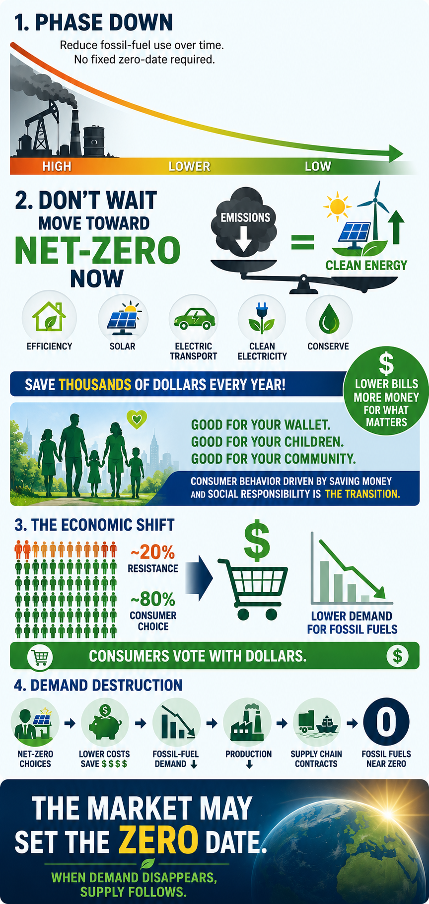
1. For this generation, I prefer net-zero carbon emissions as the immediate goal. If someone isn’t already moving toward net-zero, I think they should start now. We don’t need to wait for a theoretical future phase-out date to begin reducing emissions.

2. As both a climatologist and an economist, I’m not convinced that setting a specific date for the complete elimination of fossil fuels is ultimately what matters. In the U.S., roughly 20% of the population appears ideologically committed to policies that would accelerate climate change. Nothing I say or do is likely to change that.

But that still leaves roughly 80% of the population—and I think economics is going to do much of the work.

Right now, perhaps only ~0.5% of Americans are seriously attempting a structured net-zero lifestyle through continuous behavioral reductions and intentional balancing. As more people discover that net-zero can actually save them thousands of dollars a year while also leaving a better environment for their children and grandchildren, I expect consumer behavior to change.

When the remaining ~79.5% begin voting with their dollars, fossil-fuel demand will fall. That creates demand destruction, which ultimately means suppliers will have less and less reason to produce fossil fuels.

So, ironically, I don’t think we necessarily need to establish the exact date when fossil fuels reach zero. The market may establish that date for us. The “complete stop” happens when there is no longer sufficient demand to sustain the fossil-fuel supply chain.

Question:

When you use the term net zero is it with the understanding that the “net” component allows continuous greenhouse gas emissions under the assumption that unproven removal technologies or flawed offsets will balance them out later, delaying necessary fossil fuel phaseouts?

Net zero is a contentious term within my community and I want to be clear that I understand how you see and apply it.

Reply:

That’s an important distinction. When I use the term net-zero, I’m talking about it at the personal/lifestyle level, and I am not using “net” to justify continuing to emit greenhouse gases while assuming that unproven technologies or questionable offsets will clean up the problem later.

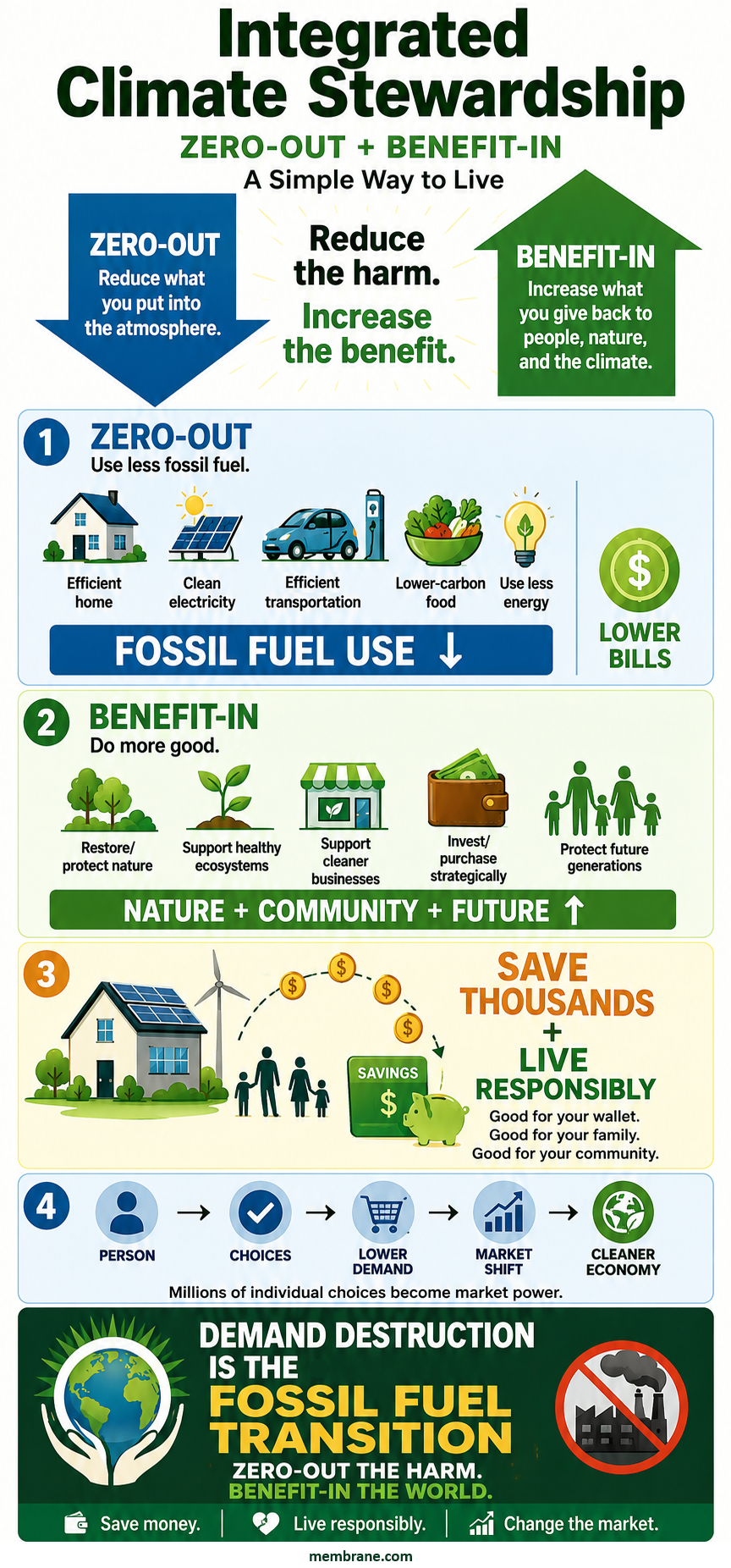
What I mean is closer to “Holistic Net-Zero Living” or “Integrated Climate Stewardship”: reducing and, wherever realistically possible, zeroing out the emissions associated with my own lifestyle first, while also taking responsibility for the impacts I can’t immediately eliminate.

For me, that means a 360-degree carbon strategy:

ZEROING OUT / STRUCTURAL DECARBONIZATION

  • Electrifying transportation and home energy
  • Increasing energy efficiency
  • Using clean electricity
  • Reducing fossil-fuel consumption as close to zero as practical
  • Reducing high-carbon consumption, including dietary choices

BEYOND MY DIRECT FOOTPRINT

  • Supporting ecosystem restoration and conservation
  • Protecting forests and biodiversity
  • Supporting businesses and technologies that accelerate decarbonization
  • Using my purchasing and investment decisions to create economic demand for cleaner alternatives

So I’m not saying, “Keep emitting and someone will remove it later.” Quite the opposite. The first priority is eliminating the emissions themselves.

I think of the “net” component as recognizing that an individual cannot instantly eliminate every indirect emission associated with modern life. Rather than pretending those emissions don’t exist, I try to compensate through additional positive actions while continuously working to reduce the underlying footprint.

Ultimately, my goal isn’t simply to achieve a favorable carbon-accounting number. It’s to change the way I live so that my actual fossil-fuel demand approaches zero—and to use my economic choices to help make that transition happen systemically.

That’s why I sometimes think “holistic net-zero living” or “integrated climate stewardship” communicates what I mean better than simply saying “net-zero.”

Question:

Why continue using the language of ‘net zero’? What economic model do you see best aligns w/ what you have outlined?

Reply:

Haaha… good questions.

A: I’m actually in the process of writing the paper that officially changes my language from “net-zero” to “Integrated Climate Stewardship.” So thank you for pushing me on that. I think the new terminology better captures what I’ve been trying to describe.

B: I’m also working on the economic model, and that one is considerably trickier—not because of the terminology, but because AI is changing the underlying economics so rapidly.

I see AI as a double-edged sword. On one edge, as AI replaces more human labor and productivity, the human contribution to economic production could eventually become a much smaller share of GDP. AI may also be capable of producing enormous amounts of economic value with far less energy per unit of output than traditional human labor and many existing production systems.

But the other edge of that sword is wealth distribution.

If the ownership of AI, capital, and productive capacity becomes increasingly concentrated, we could see extraordinary productivity growth occurring alongside increasingly unjust wealth inequality. We could potentially solve one problem—resource and energy efficiency—while creating another: who actually owns and benefits from the productivity?

That’s the economic model I’m wrestling with now: how do we build an economy where AI-driven productivity, decarbonization, consumer savings, and environmental stewardship reinforce each other while the resulting wealth is broadly distributed?

That may ultimately be a much bigger economic question than the climate transition itself.

Question:

Have you been sitting with the economic of degrowth in all of this then? Sounds like there is that tension in what is being considered.

Reply:

Yes. I’ve been sitting with the economics of degrowth quite a bit. And I think there’s an interesting tension here.

Traditional capitalism is fundamentally tied to population growth, human labor, productivity, and consumption. But AI potentially breaks that relationship. If technology increasingly replaces human labor, then economic growth can continue—even accelerate—while the economic value of human labor declines, perhaps dramatically.

So I’m not sure the future necessarily looks like “degrowth.” It may be something stranger: exponential technological growth occurring alongside declining human labor demand, an aging population in the developed regions of the world, and potentially declining population worldwide.

That raises a much bigger question: if human labor is no longer the primary engine of economic value, what exactly are we trying to maximize—and how should the economy distribute the benefits of that productivity?

That’s the economic model I’m wrestling with right now.

Question:

What about lands and waters in these considerations?

Can we agree that what we need must be either mined or grown?

Raw materials come from somewhere with significant externalities — often left out of economic theory.

My other issue is the assumptive ghost of interest-bearing-debt as a driver of unnecessary growth.

Reply:

Yes—and I think land, water, and raw materials have to be part of the model. My initial modeling, however, is pointing toward a very different problem than the one we traditionally assume.

If AI continues improving itself, productivity could eventually become extraordinarily resource-efficient. Very little additional human labor—and potentially much less land, water, or energy per unit of economic output—may be required for productivity and growth. At the same time, consumers could be forced to consume much less because their income from labor is declining. And as solar and other clean-energy technologies continue becoming cheaper, the pressure for some forms of mining and extraction could decline as well.

That brings me back to your point about interest-bearing debt. I think sovereign debt may become the critical part of the equation.

Productivity gains and abundant cheap clean energy are profoundly deflationary. Deflation sounds wonderful for consumers in theory—but not if it is accompanied by collapsing labor income. You could have falling costs and prices while households simultaneously lose the purchasing power needed to buy anything.

Now add governments facing enormous debt obligations while their traditional tax base is shrinking because human labor is becoming less economically valuable. Governments could increasingly rely on interest-bearing debt to finance poverty reduction, redistribution, and some form of basic income.

And that creates a potentially nasty feedback loop: AI-driven productivity → declining labor income → shrinking tax base → rising sovereign debt → greater reliance on monetary expansion → inflationary pressure.

Historically, severe sovereign debt problems have sometimes been resolved through substantial currency devaluation and inflation. I’m not saying hyperinflation is inevitable—but it is one of the risks I’m now modeling.

The really strange possibility is that we could simultaneously have exponential productivity, increasingly abundant cheap energy, falling costs of production—and increasing economic hardship for ordinary people.

In other words, the problem may not ultimately be whether the planet can produce enough. It may be whether humans can maintain enough income, purchasing power, and economic agency to participate in the abundance that AI creates.

That, to me, is where the economic model gets really interesting.

bookmark_borderRocky Rex Climate Climax

One way into discussing climate change as a whole is to refer to the water cycle, because most people learned about it at school.

The water cycle is now supercharged by extra heat in the oceans.

Warmer seas produce more evaporation – and that extra water vapour* carries the extra heat high into the air. The water vapour then releases the extra heat into high-altitude air as it condenses to make clouds. So weather systems are becoming more energetic, more chaotic. Like other aspects of the climate systems, the water cycle seems to be creating more extremes – prolonged droughts, and also sudden huge rainfall events.

*7% more water vapour for each extra 1 C degree of average global temperature, so we’ve added about 10% at this point. Changes of state (such as evaporation and condensation) involve lots of heat – in physics this is called latent heat.


Our system gives no value to global commons such as the atmosphere or the oceans, because they are not seen as “scarce commodities”. One oak tree does not matter, because there are vast numbers of oak trees.

Pumping sewage into the sea doesn’t matter, because the sea is too big for it to matter.

Pumping CO2 into the air doesn’t matter, because the air is limitless.*

This is a mythological view of the world, and generally people prefer myths to facts, because facts don’t obey wishes.

*In fact if there was a lift that could travel vertically at the speed of a fast car, within minutes you’d need breathing equipment.

— Rocky Rex


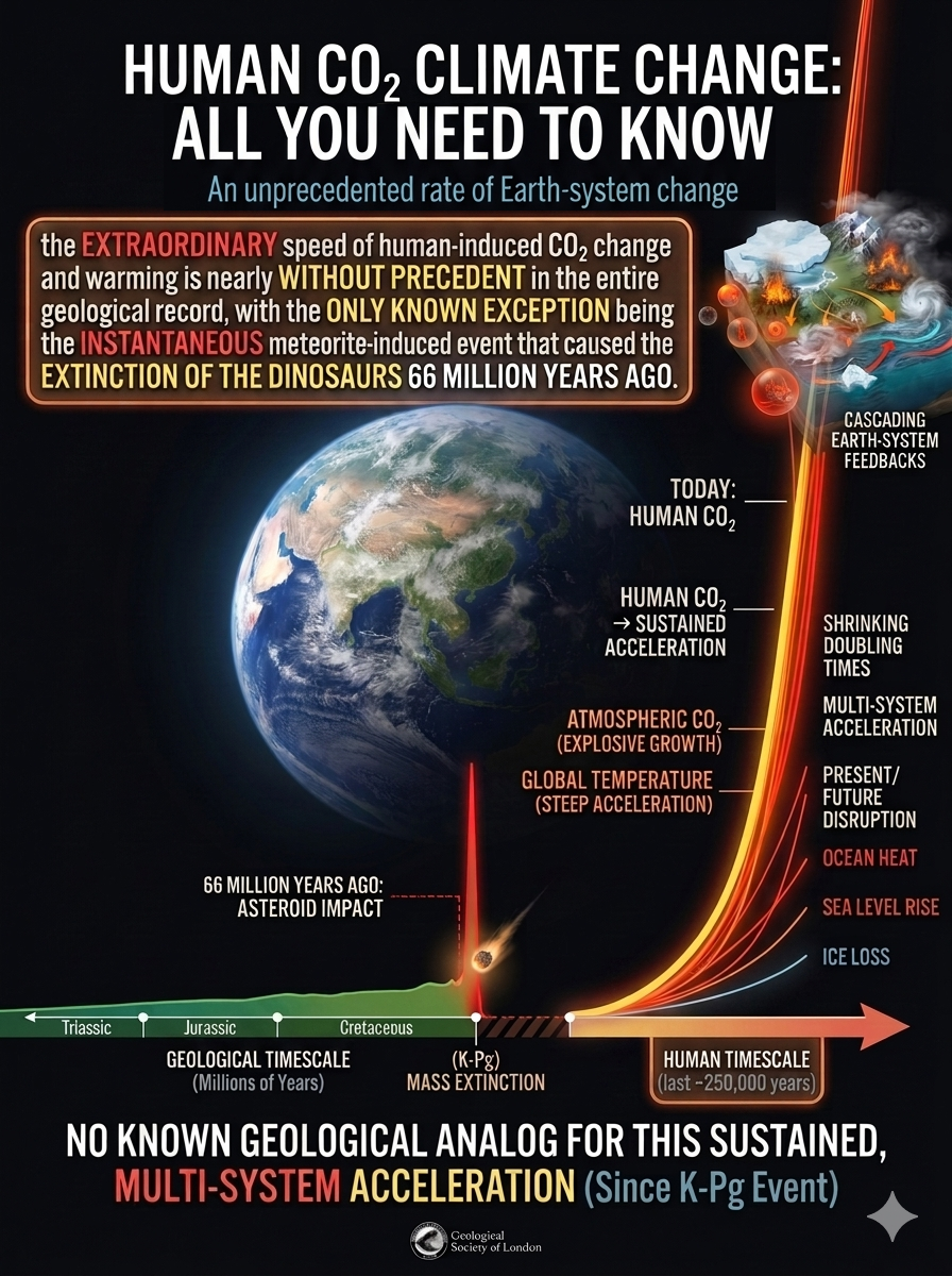
Human CO2 Climate Change: All You Need to Know
An unprecedented rate of Earth-system change.

The Geological Society of London (the UK’s expert association of professional geologists since 1807) says:

” ….the current speed of human-induced CO2 change and warming is nearly without precedent in the entire geological record, with the only known exception being the instantaneous, meteorite-induced event that caused the extinction of non-bird-like dinosaurs 66 million years ago” (H/T Rocky Rex)

We’ve arrived at a very similar observation in our own work, but I don’t think I’ve seen it stated this clearly—or published elsewhere. Thanks, Rocky, for helping to illuminate it.

Juxtapose the two and let me know whether the comparison can be communicated more effectively.

Multiple climate indicators now point to rates of warming-related disruption far beyond those observed during the modern instrumental era.

There is no well-established geological analog for a sustained, multi-variable, decade-scale pattern of accelerating change across the full Earth system at the resolution available in contemporary observations. If sustained, this may represent one of the most abrupt large-scale climate transitions in Earth’s geological history.

Rocky replied:

I’ve been citing that for a long time, and I’m always impressed by how many people can totally ignore it. It’s very much the scientific version of “The Good Ancestor” poem, it should hit people between the eyes and wake them up. All the signs are that we are entering an abrupt climate change process. Have I told you this true story before?

In the mid 1950s, Russell Coope was looking for a PhD project after graduating as a geologist. He noticed beetle remains in ice age deposits in a gravel pit in the UK Midlands. His supervisor, Prof Fred Shotton, said something like: “I expect they are just modern beetles that have got stuck to the surface.” Fred was wrong – a rare event.

Coope decided to base his PhD on recording what kinds of beetles there were in different ice age deposits, to see where it led. He discovered that the mix of beetles was linked to the temperatures at that time.

He did this by comparing his layer-by-layer collections with collections of beetles from different places in the modern world – beetles happen to evolve very slowly, so the actual variety of beetles hasn’t changed much over the last million years or so.

As his research proceeded, Coope was shocked to find that the beetles showed that at times, during the ice ages, temperatures had changed significantly in just a few decades – his beetles showed that the Earth’s climate is not fundamentally stable.

He had discovered abrupt climate change events, a previously unknown phenomenon. Geologists had always assumed that most processes were slow.

I had the good fortune to be a student in Coope’s palaeontology lectures long ago…. and also in Fred’s physical geology lectures. (In 1943, Fred Shotton was involved in a secret project that produced geological maps of certain beaches in northern France…… that’s a movie that should be made by someone)

“We are messing with the trigger that causes climate change….the outcome is likely to be ferocious.”

– Professor Russell Coope (1930-2011)

Russell Coope and his ice age beetles https://www.youtube.com/watch?v=xMyt-UbcUQo

Russell Coope on fossil beetles in the Cromer Forest-bed at Happisburgh, Norfolk, UK

YOUTUBE.COM

Russell Coope on fossil beetles in the Cromer Forest-bed at Happisburgh, Norfolk, UK

Russel

The Human Induced Climate Change Experiment

Warming → Feedback Activation → Feedback Coupling → Amplification → Tipping-Point Threshold → Cascade

The climate system is not simply warming—it is changing how it responds to that warming. Coupled climate feedbacks are becoming one of the most consequential dimensions of climate risk in the 21st century because they amplify changes and connect individual tipping-point pathways into larger cascading effects.

The longer warming persists, the more climate feedbacks become active. As these feedbacks interact, we are already observing nonlinear responses, amplification, and cascading impacts across the climate system. Hundreds of feedback mechanisms have been identified, and many can couple and reinforce one another, contributing to the accelerating pace and increasing magnitude of climate change—The Domino Effect.


by Daniel Brouse, Sidd Mukherjee, and Rocky Rex

Can Anthropogenic Global Warming Be Proven?

Yes.

The isotopic signature of atmospheric carbon dioxide provides direct evidence.

Fossil carbon is depleted in 13C and contains essentially no measurable 14C (radiocarbon), because 14C decays over thousands of years.

Observed atmospheric trends show:

  • A measurable decline in the 13C/12C ratio
  • A measurable decline in atmospheric 14C concentration
  • A measurable decline in atmospheric O2 concentration

These shifts form a remarkably consistent fingerprint.

The carbon isotopes tell us where the additional carbon is coming from. Fossil fuels were formed from ancient biological material and therefore have a characteristic isotopic signature: relatively little 13C and virtually no 14C. As fossil carbon is added to the atmosphere, the atmospheric CO2 isotope ratios shift in precisely the direction expected from fossil-fuel combustion.

The decline in atmospheric oxygen provides an independent piece of evidence.

When fossil fuels are burned, carbon combines with atmospheric oxygen:

C + O2 → CO2

The process consumes O2 and produces CO2. Because the additional atmospheric CO2 is accompanied by a measurable decline in atmospheric O2, the observations are consistent with large-scale combustion of carbon rather than simply a redistribution of carbon through the natural carbon cycle.

This is especially important because the ocean, vegetation, and atmosphere continuously exchange carbon and oxygen. Natural processes can move carbon between reservoirs, but they do not explain the simultaneous long-term pattern of rising CO2, falling O2, declining 13C/12C, and declining radiocarbon.

The four observations reinforce one another:

Rising atmospheric CO2
↓
Declining 13C/12C
↓
Declining 14C
↓
Declining atmospheric O2

Together, these measurements provide a chemical and isotopic fingerprint of fossil-carbon combustion.

Volcanoes do not produce the observed isotopic pattern, and the natural carbon cycle cannot account for the simultaneous changes in the required direction and magnitude.

The molecules carry their own fingerprint—and the atmosphere is preserving the evidence in both carbon and oxygen.


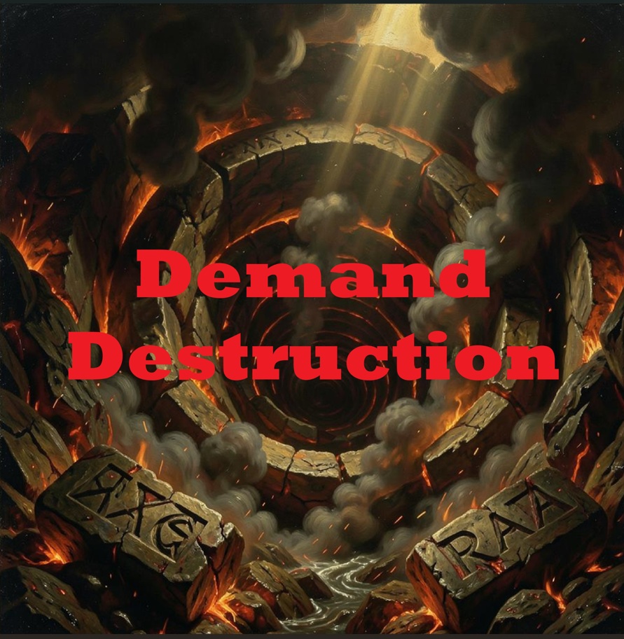
Demand Destruction Album Cover

Demand Destruction


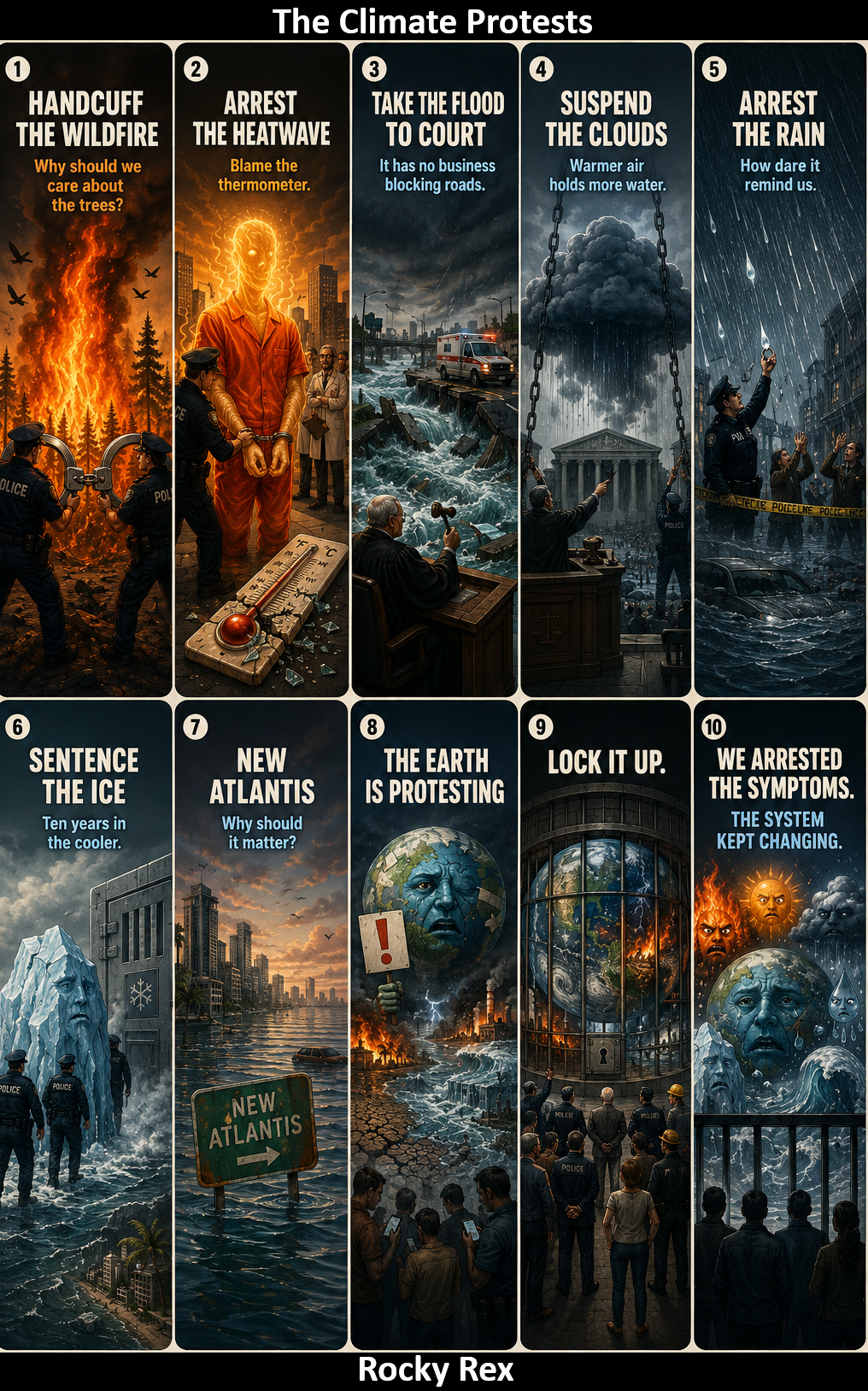
THE CLIMATE PROTESTS

by Rocky Rex

“Handcuff the wildfire.

Why should we care about the trees?

What did the birds ever do for us?

Dress the heatwave in an orange jumpsuit.

It is probably a fault in the thermometer anyway.

These scientists – what do they know?

Take the flood to court.

It has no business blocking roads, or sweeping away bridges.

What if an ambulance was stuck on the wrong side of the river?

Give the clouds a suspended sentence.

They are trying to remind us that a warmer world has wetter air. They should go and tell China, not us.

Arrest the rain.

How dare it remind us that the climate is changing?

Let’s pretend it always rained like this.

Sentence the melting ice to 10 years in the cooler.

Why does it matter if the sea floods Bangladesh?

And Miami can be the New Atlantis.

The Earth is protesting?

We are not interested – just lock it up.”


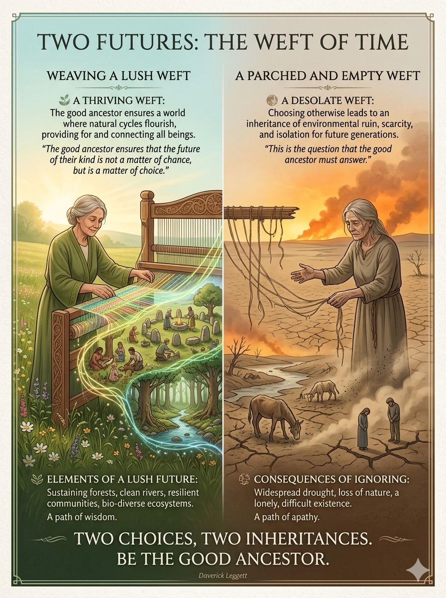
The Good Ancestor

A poem by Daverick Leggett

Every day I walk a hundred years
to the hill where my great, great granddaughter sits.
I carry words of blessing
and reach to touch her back.

But feeling me near she turns,
sad-eyed and heavy with grief.

“What was it like?” she asks,
“when the great whales swam,
when the birds sang you awake,
when the rains came soft,
and the soil smelled sweet underfoot?”

And the blessings
catch in my throat.

On darker days she turns,
her famished face charred, and eyes
sunk in their bony orbits,
burn with curses.

And the blessings
froth at my mouth
with the poisonous
spume of betrayal.

On the darkest of all days
I walk the hundred years
and find no one there.

Let today be the bright day.
Let today be the bright day
I lay my hand upon her back.

And, feeling me near, she turns
and blesses me, saying,

“Your love was fierce enough,
sweet ancestor,
your love was fierce enough.”


About Rocky Rex

I was a science teacher for a long time – and I taught geology when I could. Rocky Rex began as a poster on my lab wall….I was given a T Rex poster, and as soon as I pinned it up I knew he was called Rocky Rex. The name just came to me, out of nowhere.

He gave a focus for information added to his notice board. He ended up making money for school funds by appearing on T-shirts, pens, key-rings etc.

It wasn’t long before some of the other staff started calling me Rocky. This was all long before the internet existed, but when social media appeared it just seemed obvious that my avatar would be Rocky Rex. I like keeping my online stuff slightly disconnected from my offline life. [I actually did a physics degree, but we had to take an “additional science” course in the first year, so I chose geology. It was the same geology course taken by those doing a joint degree in geology and archaeology. ]

bookmark_borderThe Strange and Hidden Feedback Network: Chaos Theory and the Acceleration of Climate Change

by Daniel Brouse

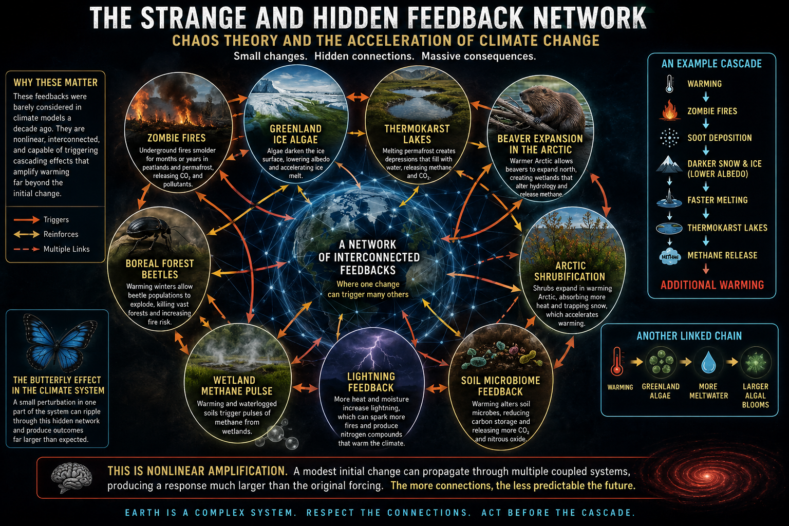
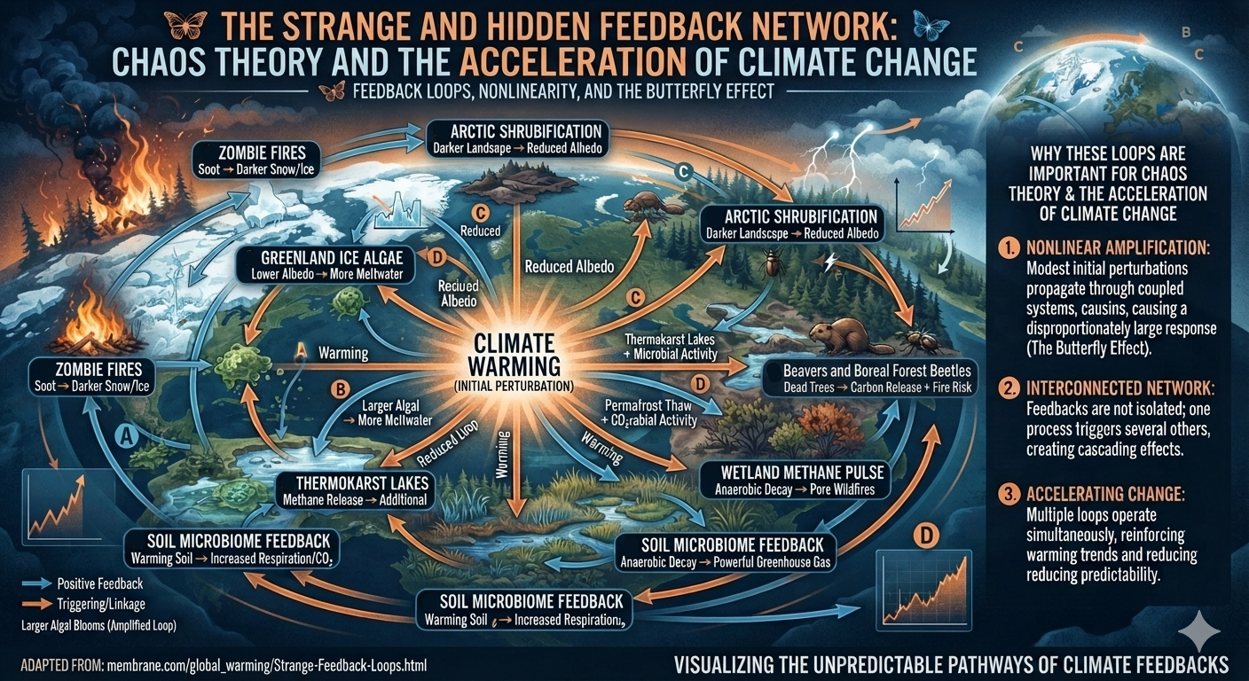
Some of the most fascinating—and concerning—climate feedback loops are ones that were barely considered in climate models a decade ago. They illustrate how a relatively small change can trigger a cascade of nonlinear responses, making them particularly relevant from a chaos theory perspective.

Chaos Theory and the Acceleration of Climate Change

Climate change isn’t just one feedback causing another.

It’s becoming a network of interacting feedbacks where seemingly unrelated processes reinforce each other in ways that traditional linear thinking struggles to capture.

Our newest infographic explores some of the Earth’s most unusual and recently recognized climate feedbacks, including:

🔥 Zombie Fires
🟢 Greenland Ice Algae
🏞️ Thermokarst Lakes
🦫 Arctic Beaver Expansion
🪲 Boreal Forest Beetles
🌿 Arctic Shrubification
💨 Wetland Methane Pulses
⚡ Lightning Feedback
🦠 Soil Microbiome Feedback

These systems don’t operate independently.

A small change can trigger multiple connected responses that amplify one another—a climate-scale example of the Butterfly Effect.

For example:

Warming → Zombie Fires → Soot on Ice → Lower Albedo → Faster Melting → Thermokarst Lakes → Methane Release → More Warming

This is nonlinear amplification: modest initial changes propagating through interconnected systems to produce responses far larger than the original disturbance.

As these hidden connections strengthen, predicting climate behavior becomes increasingly difficult using simple cause-and-effect models.

Understanding the network is becoming just as important as understanding the individual feedbacks.

🌍 Every new connection matters.

1. Zombie Fires (Overwintering Peat Fires)

Feedback loop:

  1. Higher temperatures → more drought.
  2. Peat ignites during summer fires.
  3. Fire smolders underground all winter.
  4. Fire re-emerges the following spring.
  5. Vegetation and insulating peat disappear.
  6. Permafrost thaws.
  7. Ancient carbon and methane are released.
  8. More warming → more fires.

These fires can survive beneath snow because peat acts like charcoal, insulating the combustion. They’re becoming increasingly common across Canada and Siberia as warmer, drier conditions expand.


2. Greenland Ice Algae

Perhaps one of the strangest biological feedbacks.

Feedback loop:

  1. Warmer summers melt snow.
  2. Microscopic algae bloom on exposed ice.
  3. Dark pigments reduce ice reflectivity (albedo).
  4. More sunlight is absorbed.
  5. Ice melts faster.
  6. More liquid water supports additional algae.

Researchers call this biological darkening. In parts of Greenland’s “Dark Zone,” algae have become a measurable contributor to increased melt.


3. Thermokarst Lakes

One of the least intuitive feedbacks.

Feedback loop:

  1. Permafrost begins thawing.
  2. Ground collapses into depressions.
  3. Lakes form.
  4. Water conducts heat much better than frozen soil.
  5. Deeper permafrost melts.
  6. Ancient organic carbon decomposes.
  7. Methane bubbles escape.
  8. Methane accelerates warming.

Small lakes become “hot spots” that can emit disproportionately large amounts of methane.


4. Beaver Expansion in the Arctic

As northern regions warm:

  • beavers move farther north,
  • they build dams,
  • ponds trap warm water,
  • warm water melts surrounding permafrost,
  • wetlands expand,
  • methane emissions increase.

An animal once considered ecologically beneficial in temperate regions becomes an unexpected amplifier of Arctic warming.


5. Boreal Forest Beetles

Cold winters historically killed bark beetles.

Now:

  • milder winters
  • more beetles survive
  • forests die
  • dead forests burn more easily
  • fires release carbon
  • soot darkens snow and ice
  • additional warming allows beetles to expand farther north.

6. Wildfire Smoke Darkening Snow

Smoke doesn’t just affect air quality.

Wildfire ash and black carbon settle on:

  • glaciers
  • Arctic sea ice
  • mountain snowpack

This lowers albedo, causing earlier melt, which exposes darker land and ocean surfaces that absorb even more solar energy.


7. Arctic Shrubification

As tundra warms:

  • shrubs invade formerly snow-covered areas,
  • shrubs absorb more sunlight than snow,
  • shrubs trap drifting snow,
  • deeper snow insulates the soil,
  • winter soil temperatures rise,
  • permafrost thaws faster.

A simple change in vegetation alters the thermal properties of the landscape.


8. Rain-on-Snow Events

Increasing winter rain instead of snow causes:

  • ice crust formation,
  • vegetation damage,
  • reduced insulation,
  • altered hydrology,
  • increased runoff,
  • greater summer drying,
  • increased wildfire risk.

This feedback connects winter weather directly to summer fire seasons.


9. Kelp Forest Collapse

Marine heat waves can eliminate kelp forests.

Loss of kelp means:

  • less carbon uptake,
  • reduced coastal cooling,
  • altered nutrient cycling,
  • warmer coastal waters,
  • additional kelp mortality.

10. Ocean Stratification

Warmer surface oceans become lighter.

This reduces vertical mixing.

Consequences include:

  • less oxygen reaching deep water,
  • reduced nutrient upwelling,
  • warmer surface layers,
  • marine heat waves become more persistent,
  • coral bleaching,
  • weaker biological carbon pump.

11. Wetland Methane Pulse

Heavy rainfall creates:

  • saturated soils,
  • oxygen-poor conditions,
  • methanogenic microbes,
  • increased methane emissions,
  • additional warming.

Ironically, wetter conditions can increase greenhouse-gas emissions from wetlands.


12. Glacier Elevation Feedback

As glaciers melt:

  • their surfaces sink,
  • lower elevations are warmer,
  • melting accelerates,
  • glaciers descend farther into warmer air,
  • retreat speeds up.

Greenland exhibits this effect over large areas.


13. AMOC Freshwater Feedback

Greenland meltwater freshens the North Atlantic.

Fresh water is less dense, reducing deep-water formation.

This can alter ocean circulation, redistribute heat, and change regional weather patterns. Some studies suggest this may also increase subsurface warming near marine-terminating glaciers, enhancing ice-sheet melt.


14. Lightning Feedback

Warmer air produces:

  • more atmospheric moisture,
  • greater instability,
  • more lightning,
  • more wildfire ignitions,
  • greater carbon emissions,
  • additional warming.

Recent studies indicate lightning activity is increasing in parts of the Arctic, where lightning was historically uncommon.


15. Soil Microbiome Feedback

Warmer soils stimulate microbial activity.

Microbes decompose organic matter faster, releasing:

  • CO₂
  • methane
  • nitrous oxide

These gases further warm the atmosphere, increasing microbial activity even more.


Why these are important for chaos theory

What’s striking is that these feedbacks don’t operate independently. They form an interconnected network in which one process often triggers several others. For example:

  • Warming → zombie fires
  • Zombie fires → soot deposition
  • Soot → darker snow and ice
  • Darker ice → faster melting
  • Faster melting → thermokarst lakes
  • Thermokarst lakes → methane release
  • Methane → additional warming

Likewise:

  • Warming → Greenland algae
  • Algae → lower albedo
  • Lower albedo → more meltwater
  • Meltwater → larger algal blooms

These interactions exemplify nonlinear amplification: a modest initial perturbation can propagate through multiple coupled systems, producing a response much larger than the original forcing (The Butterfly Effect). That networked behavior is one reason Earth-system responses can become increasingly difficult to predict with linear cause-and-effect thinking.

bookmark_borderEarth’s Thin, Changing Atmosphere: How Human Climate Change Is Reshaping the Troposphere

By Daniel Brouse
Economist & Climatologist
Membrane Domain USA
August 10, 2026

Our system gives no value to global commons such as the atmosphere or the oceans, because they are not seen as “scarce commodities”. One oak tree does not matter, because there are vast numbers of oak trees.

Pumping sewage into the sea doesn’t matter, because the sea is too big for it to matter.

Pumping CO2 into the air doesn’t matter, because the air is limitless.*

This is a mythological view of the world, and generally people prefer myths to facts, because facts don’t obey wishes.

*In fact if there was a lift that could travel vertically at the speed of a fast car, within minutes you’d need breathing equipment.

— Rocky Rex

Earth’s Thin, Changing Atmosphere: How Human Climate Change Is Reshaping the Troposphere

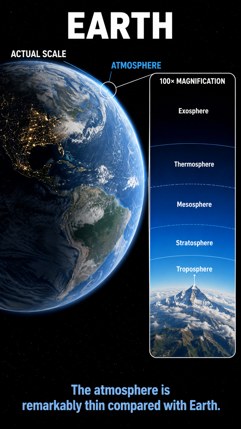
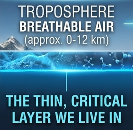
Human-driven climate change is profoundly altering the thin atmospheric layer in which we live—the troposphere. Greenhouse-gas accumulation is changing its temperature, vertical structure, moisture content, and relationship with the layers above it.

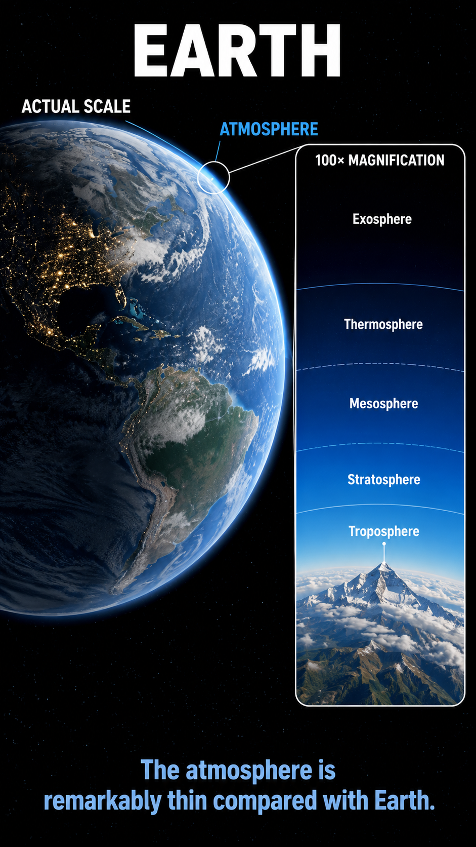
The atmosphere may look enormous in many illustrations, but relative to the size of Earth, the layer where virtually all human life and weather occur is remarkably thin. Climate change is not simply warming this layer; it is changing the structure and dynamics of the atmosphere itself.

1. The Troposphere Is Expanding

As rising greenhouse-gas concentrations warm the troposphere, the atmosphere responds dynamically by expanding. One measurable consequence is a rising tropopause—the boundary between the troposphere and stratosphere.

Observations from radiosondes and satellite GPS-radio-occultation measurements show that the tropopause has risen substantially in recent decades. In the Northern Hemisphere, studies find an average rise of roughly 50–60 meters per decade since 2000, with tropospheric warming identified as the primary driver.

This does not mean that the entire atmosphere is simply being pushed upward like a solid layer. Rather, warming changes the temperature structure and density of the atmosphere, causing the troposphere to occupy a greater vertical extent.

The result: Earth’s already-thin weather layer is expanding upward.

2. Warming Below, Cooling Above

One of the clearest fingerprints of increasing greenhouse gases is a vertical temperature contrast: the troposphere warms while much of the stratosphere cools.

This occurs for different physical reasons in the two layers. In the troposphere, increasing greenhouse gases reduce the rate at which infrared energy escapes directly to space, contributing to warming near the surface and throughout much of the lower atmosphere. In the stratosphere, increasing CO₂ enhances radiative emission to space, producing cooling.

The observed long-term cooling is strongest in the middle and upper stratosphere, where NOAA assessments attribute much of the trend to increasing CO₂ and other greenhouse gases. The lower stratosphere is more complicated: its temperature has shown little long-term global trend since the late 1990s because multiple influences—including ozone changes and natural variability—act simultaneously.

This creates a changing thermal structure across the tropopause.

That matters because temperature gradients help organize winds, atmospheric circulation, jet streams, and the movement of weather systems. Changes in the troposphere–stratosphere system can therefore propagate downward into the weather patterns experienced at Earth’s surface.

3. A Warmer Atmosphere Carries More Water

A warmer atmosphere can contain substantially more water vapor. The Clausius–Clapeyron relationship implies approximately 7% more water-holding capacity per 1°C of warming near typical atmospheric temperatures.

This does not mean that every location becomes 7% wetter. Actual atmospheric moisture depends on evaporation, circulation, precipitation, and regional conditions.

But where additional moisture is available, a warmer atmosphere can support larger amounts of water vapor and heavier precipitation.

Water vapor is itself a powerful greenhouse gas, creating an important positive feedback:

Warming → more atmospheric moisture → stronger greenhouse effect → additional warming

The same additional moisture can also increase the potential intensity of extreme precipitation because storms have access to larger quantities of atmospheric water.

In other words, climate change is altering not only the temperature of the atmosphere but also the amount of energy and water circulating through our thin atmospheric habitat.

4. The Ozone Layer Is Being Affected—But Not Simply “Compressed”

The expanding troposphere interacts with the upper troposphere–lower stratosphere (UTLS), a region where chemistry, radiation, and atmospheric circulation are tightly coupled.

Climate change can alter stratospheric temperatures, circulation, water vapor, and ozone distribution. Increasing greenhouse gases cool the stratosphere and modify atmospheric circulation, while ozone changes themselves affect stratospheric temperature and circulation.

However, it is misleading to say that the expanding troposphere simply “compresses” or “thins” the ozone layer. The ozone layer is not a rigid physical shell. Its distribution changes through interacting chemical and dynamical processes.

Importantly, the global ozone layer is currently recovering from the effects of ozone-depleting substances because of the Montreal Protocol. Climate change nevertheless continues to interact with ozone chemistry and stratospheric circulation, making the relationship between the two systems increasingly important.

5. The Bigger Picture: A Thin Layer Undergoing Structural Change

The most important point is not that climate change is merely making the atmosphere warmer.

It is reorganizing the atmosphere vertically and dynamically.

The troposphere is expanding.
The tropopause is rising.
The troposphere is warming.
Much of the stratosphere is cooling.
Atmospheric moisture is increasing as temperatures rise.
Circulation patterns are changing.
And the interaction between the troposphere, stratosphere, water vapor, and ozone is becoming increasingly important.

All of this is occurring within a layer that is astonishingly thin compared with the size of Earth.

That is perhaps the most important perspective:

We do not live on Earth beneath an enormous atmosphere. We live inside an extraordinarily thin atmospheric layer wrapped around a planet.

Human activity is now changing the physical and chemical properties of that layer on a global scale.

The atmosphere is thin.
The changes are not.

bookmark_borderThe Future of Energy Is Not Static

By Daniel Brouse
Economist & Climatologist
Membrane Domain USA
August 10, 2026

I’m not certain what the future holds. I don’t think anyone can be.

But I’m also not convinced that the future of fossil fuels can be projected simply by looking at today’s production levels and assuming they will continue indefinitely.

There is a very real possibility that economics, energy security, technological substitution, and even economic disruption could phase out fossil fuels much faster than most people expect.

In fact, some of the data already point in that direction.

The Energy Transition Is Already Moving

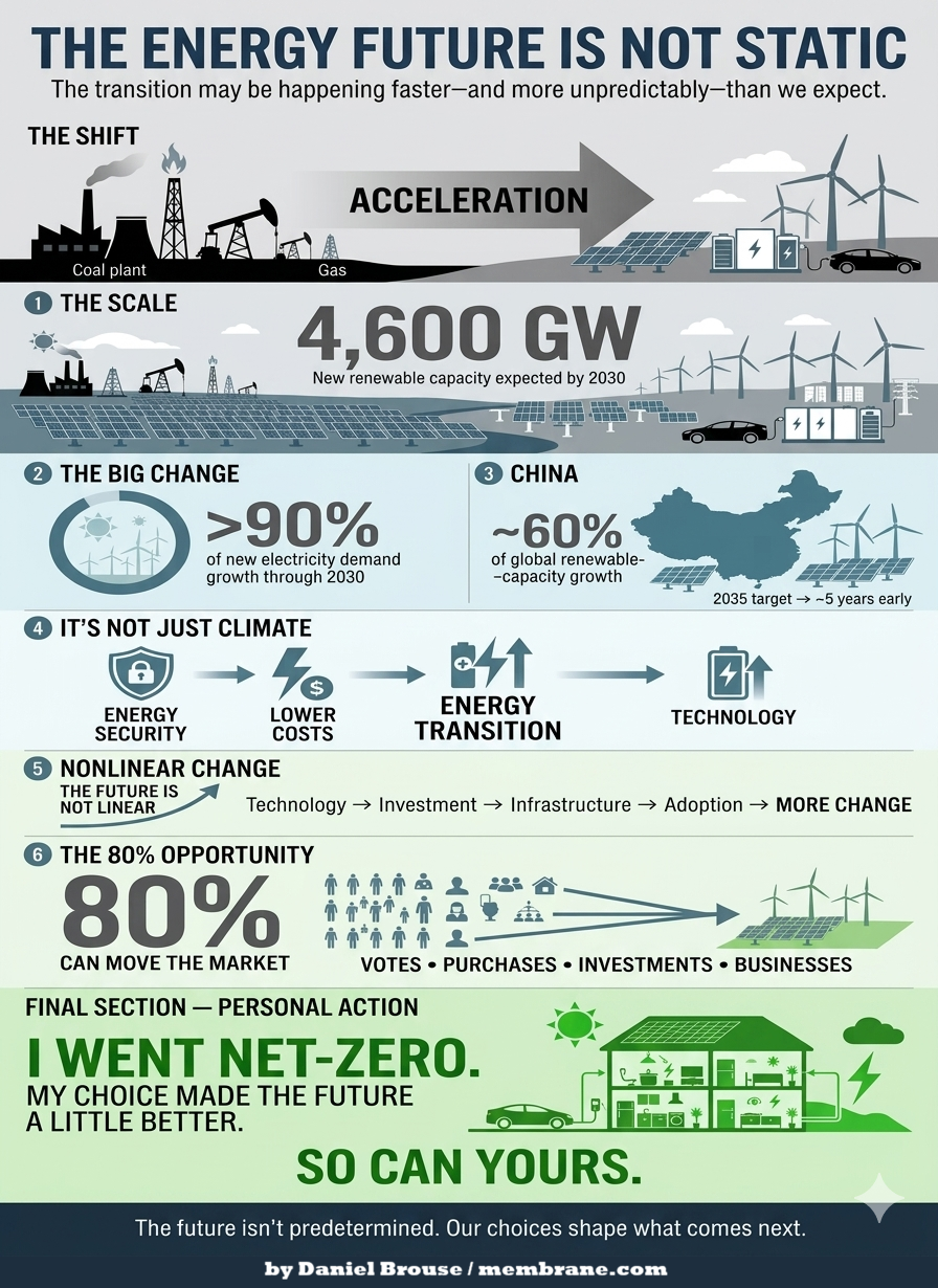
The International Energy Agency estimates that global renewable capacity will increase by roughly 4,600 GW between 2025 and 2030—an extraordinary expansion roughly equivalent to the combined current power capacity of China, the European Union, and Japan.

Solar PV is expected to account for almost 80% of that expansion.

Even more significant is what this means for the growth of electricity demand. Renewables are expected to provide more than 90% of the increase in global electricity generation through 2030.

This is not simply a distant prediction about some hypothetical future energy system. It represents an enormous investment already underway.

And the transition is happening particularly rapidly in China.

China is now responsible for nearly 60% of global renewable-capacity growth. In 2025 alone, it added roughly 314 GW of solar capacity and is on track to reach its 2035 wind-and-solar target approximately five years early.

Whatever one’s views on climate policy, these numbers are difficult to dismiss.

The global energy system is changing.

And it is changing rapidly.

This Isn’t Just About Climate Policy

There is another factor that deserves considerably more attention: energy security.

The transition away from fossil fuels is not being driven exclusively by environmental concerns. Increasingly, it is also becoming an economic and strategic imperative.

The disruption of oil and gas flows through critical transportation routes such as the Strait of Hormuz demonstrates the vulnerability inherent in an energy system dependent upon globally traded fossil fuels.

For Europe and Asia in particular, domestic renewable generation, energy storage, electrification, and efficiency increasingly represent something more than climate policy.

They are energy-security assets.

A solar panel or wind turbine doesn’t need to be transported through a geopolitical chokepoint every time it generates electricity. Once installed, domestic renewable resources can reduce exposure to international fuel-price shocks, supply disruptions, and geopolitical conflicts.

That changes the economic calculation.

And it is one reason I believe the energy transition may prove considerably more nonlinear than many conventional forecasts assume.

The Future May Be Nonlinear

I agree that we shouldn’t pretend we know exactly what the future holds.

My point is almost the opposite.

The future may be much more nonlinear than either of us can confidently predict.

Technologies don’t necessarily replace one another gradually. Once a technology becomes sufficiently cheap, reliable, scalable, and convenient, adoption can accelerate rapidly.

The same thing can happen with infrastructure.

Battery storage becomes cheaper. Electric vehicles become more capable. Solar becomes less expensive. Transmission improves. Heat pumps become more efficient. Businesses discover that electrification can reduce operating costs. Consumers begin choosing technologies that save them money.

Each development can reinforce the others.

And once enough pieces of the system change, the economics of the entire energy system can change with them.

This is why simply extrapolating today’s fossil-fuel production into the future can be misleading.

Could “Drill, Baby, Drill” Backfire?

There is an irony here.

Policies intended to expand U.S. fossil-fuel production could potentially accelerate the transition they are intended to slow if they contribute to greater volatility, geopolitical exposure, or investment in alternatives.

Consider what could happen during a serious economic downturn.

A major recession could cause substantial demand destruction. Businesses would consume less energy. Consumers would drive less and purchase fewer goods. Industrial production would decline.

Fossil-fuel consumption could fall sharply.

That would potentially undermine the very industry that policies designed around expanding fossil-fuel production are intended to strengthen.

There is no guarantee this will happen. But that’s precisely the point.

The future contains feedback loops.

Economic conditions affect energy demand. Energy prices affect technology adoption. Technology affects investment. Investment affects infrastructure. Infrastructure affects energy prices and security. Geopolitical events affect all of them.

The result is a system capable of changing much faster than a simple linear projection would suggest.

This Isn’t an All-or-Nothing Choice

I’m not trying to create another online debate.

I’m simply pointing out that the data show a transition already underway—and its speed is anything but static.

And perhaps the most important point is that this isn’t an all-or-nothing proposition.

Every increment of transition matters.

Every electric vehicle displaces some gasoline consumption. Every solar panel replaces some electricity that otherwise might have come from fossil fuels. Every efficiency improvement reduces energy demand. Every battery installation makes intermittent renewable energy more useful. Every business that electrifies reduces some exposure to fossil-fuel prices.

The more we transition, the more reasonable—and manageable—the future becomes.

We don’t need to transform the entire energy system overnight.

We need to keep moving.

Technology Is Changing More Than Energy

There is another reason I remain optimistic.

Ironically, AI and rapidly advancing technology are accelerating climate science at a pace that may eventually rival the acceleration of climate change itself.

Research that once took years can increasingly be explored in hours.

Large datasets can be analyzed in ways that weren’t previously practical. Relationships between variables can be identified more quickly. Models can be tested, refined, and compared at extraordinary speed.

I’ve been able to identify hundreds of interacting feedbacks and relationships that weren’t even being seriously considered just a few years ago.

That doesn’t mean every hypothesis will be correct.

It means our ability to investigate complex systems is expanding extraordinarily quickly.

And that gives me reason for optimism.

Humans have an extraordinary capacity to adapt, innovate, and solve difficult problems—especially when we are sufficiently motivated to do so.

The future is not predetermined.

What we do now can still make an enormous difference in what comes next.

The 80% Question

A final thought concerns something that initially struck me as particularly concerning.

Roughly 20% of Americans appear to be actively fighting the energy transition.

At first, I found that almost dumbfounding. I expected the number to be closer to less than 2%.

But there is another way to look at it.

That still leaves roughly 80% of the population.

And if that 80% chooses to act—through voting, investment, purchasing decisions, business decisions, and simply choosing where to spend their dollars—the market can move remarkably quickly.

We don’t necessarily have to fight the remaining 20%.

We can vote with our dollars.

Markets respond to demand.

If enough consumers and businesses choose alternatives, capital will follow. Manufacturers will respond. Infrastructure will change. Companies will adapt.

And eventually, the fossil-fuel industry will have to adapt as well—or gradually lose market share.

That is the power of an energy transition driven not only by government policy, but by millions of individual economic decisions.

My Choice. Your Choice. Our Future.

I went net-zero years ago.

If I can do it, anybody can.

I don’t claim that my individual decision changed the world.

But my choice made the future a little better than it otherwise would have been.

And so can yours.

The future of energy isn’t predetermined by today’s production numbers, today’s political battles, or today’s assumptions.

It will be shaped by billions of decisions made by consumers, businesses, investors, engineers, scientists, and governments.

Some of those decisions will be political.

Many will be economic.

Some will be technological.

And countless others will be personal.

That’s why I don’t think the question is whether we can predict exactly what the energy system will look like in 10, 20, or 30 years.

We can’t.

The more important question is:

What direction are we moving—and how much can our choices influence where we ultimately arrive?

The transition is already underway.

Its speed is accelerating.

And the future is still ours to shape.

bookmark_borderScience Is Science: Confronting Denialism and Ecofascism

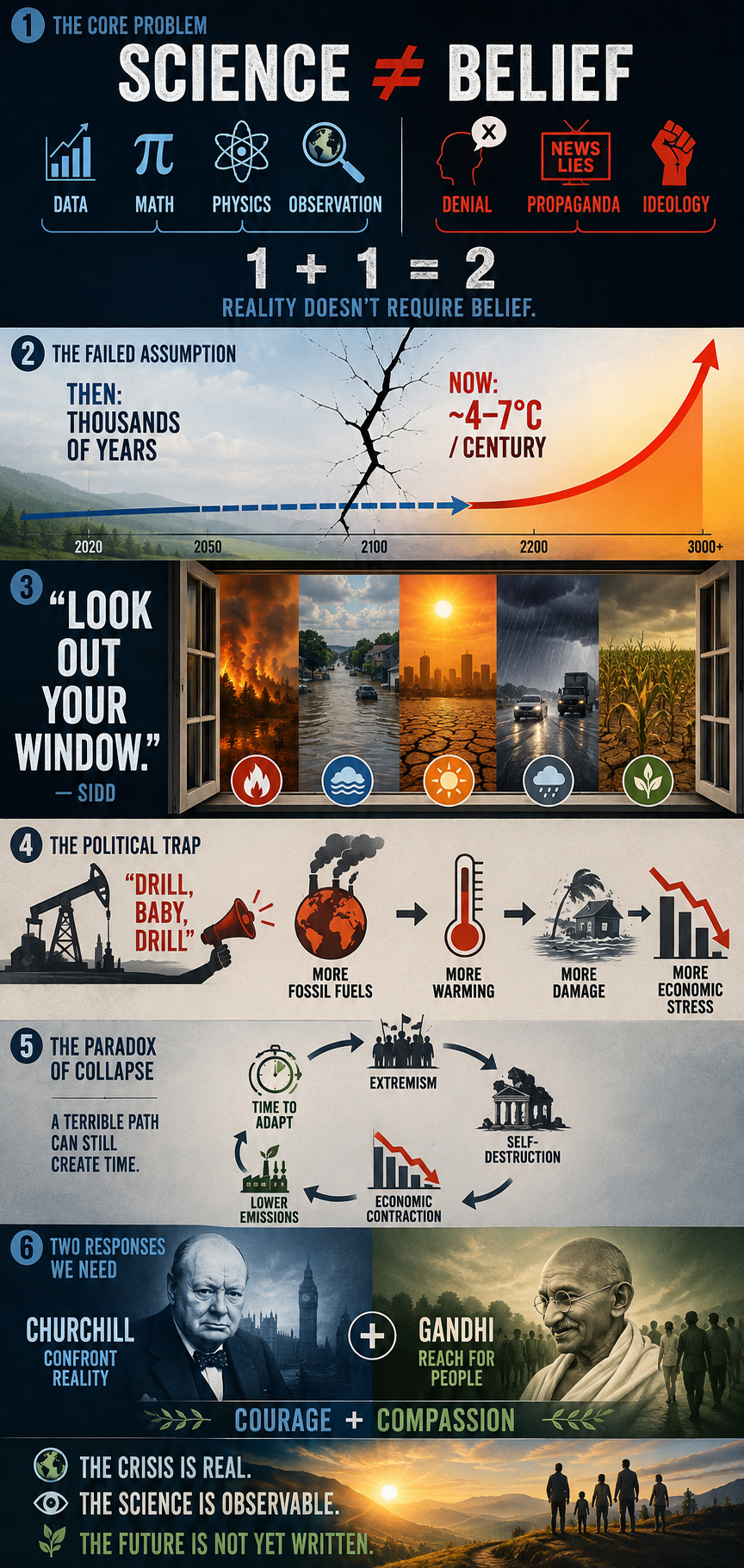
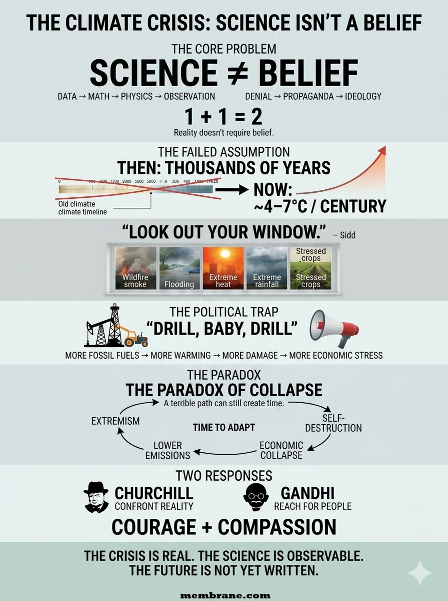
About Denialism and Ecofascism: Science Is Science

The Observation
Glad to know you’re watching out! At the same time, this divisiveness—when we desperately need everyone to pull together because it’s a CRISIS, right?—makes me somehow deeply sad.

That’s a big job right there… How do we reach those who seem furthest away from any kind of understanding? We need both a Winston Churchill and a Mahatma Gandhi in this endeavor…

The Response
Agreed. Both denialism and ecofascism are ideologies that ultimately defy logic. In very different ways, they can become a kind of combination of self-destruction and destruction of others.

I’ve spent years battling misinformation, propaganda, and rhetoric. To the best of my knowledge, neither Sidd nor I have successfully converted—or even educated—a single committed denier. Climate science has somehow been transformed into a “belief” system. But science has nothing to do with belief. 1 + 1 = 2. If someone refuses to “believe” that, what exactly can you do?

From the beginning, our work has been based on observations, data, mathematics, and the laws of physics. So yes, I think this is at the heart of the crisis. When we started this work, we genuinely believed humanity would eventually take action. We thought we had thousands, if not tens of thousands, of years to adapt. That was the one thing we got wrong.

A couple of years ago, after explaining my continuing attempts to reach climate deniers, I asked Sidd what we could possibly do. His response was essentially, “Dude, just tell them to look out their window.” It sounds simplistic, but there is profound truth in it. The consequences are becoming increasingly difficult to deny.

Since then, we’ve had to rebuild much of our modeling. A +4°C world within thousands of years is no longer the worst-case scenario we worry about. The possibility of 4–7°C of warming within a century has become a much more serious concern in our work.

And then there is the political dimension. The rise of white-nationalist and authoritarian governments in the U.S. and elsewhere has made an already difficult problem considerably harder. Paradoxically, though, history offers one small reason for hope: fascism ultimately fails. It is inherently self-destructive.

The “drill, baby, drill” mentality is economically and environmentally self-defeating. A severe economic contraction could, ironically, buy humanity some time for adaptation while drastically reducing emissions. That is hardly the future anyone should want, but history has repeatedly demonstrated that systems built on extremism and authoritarianism eventually consume themselves.

So yes—we desperately need both the Churchill and Gandhi dimensions: the willingness to confront reality without flinching, and the willingness to keep reaching for people rather than giving up on them. I’m just not sure humanity has ever faced a crisis where we needed both quite this badly.

bookmark_borderThe Humidity Paradox: Why a Warmer Atmosphere Is Getting Wetter—and Drier at the Same Time

by Daniel Brouse

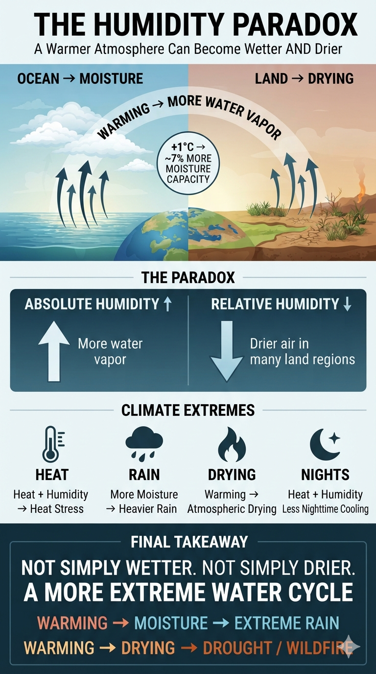
Absolute humidity—the total amount of water vapor in the air—is increasing globally as the climate warms. The fundamental physics is straightforward: according to the Clausius–Clapeyron relationship, warmer air can hold substantially more water vapor. For every 1°C (1.8°F) of warming, the atmosphere’s water-holding capacity increases by roughly 7%.

As human-caused greenhouse gas emissions raise global temperatures, evaporation from the oceans and land surface increases, adding more water vapor to the atmosphere. This creates an important distinction, however: the atmosphere can contain more water vapor even while relative humidity declines in many regions.

The Humidity Paradox

Absolute humidity measures how much water vapor is actually present in the air.

Relative humidity measures how close the air is to saturation relative to the maximum amount of moisture it could hold at that temperature.

Because warmer air has a rapidly increasing moisture capacity, these two measurements can move in different directions.

Over Much of the World’s Land

Relative humidity has declined across many continental regions. Land surfaces are warming faster than the oceans, particularly in already-dry and semi-arid regions. As temperatures rise, the atmosphere’s capacity to hold water vapor can increase faster than the actual moisture supplied by evaporation.

The result is a paradoxical combination:

More water vapor in the atmosphere + lower relative humidity = a warmer, thirstier atmosphere.

This can increase atmospheric drying demand, soil-moisture loss, vegetation stress, drought intensity, and wildfire risk.

Several regions show particularly pronounced drying trends:

  • American West and Southwest: Rapid warming is increasing atmospheric moisture demand faster than water availability in many areas, intensifying drought and wildfire conditions.
  • Interior South America: Parts of the Amazon Basin and surrounding interior regions are experiencing declining relative humidity as warming and land-use change affect moisture recycling.
  • Mediterranean Basin and Southern Europe: Declining relative humidity contributes to stronger atmospheric drying, soil desiccation, and more severe heat and drought conditions.
  • Southern Africa and Central Asia: Large continental interiors are increasingly exposed to atmospheric drying because warming is increasing moisture demand faster than local moisture supplies can compensate.

Over Oceans and Moisture-Rich Regions

Over much of the ocean, relative humidity is more stable because evaporation provides a continuing source of atmospheric moisture. In some regions, relative humidity can increase because of ocean warming, atmospheric circulation changes, and enhanced moisture transport.

The tropical oceans are especially important. Their vast warm-water surfaces provide enormous quantities of moisture to the atmosphere, helping maintain high humidity and supplying the water vapor that can fuel intense precipitation and tropical cyclones.

In the Arctic and other high-latitude regions, declining sea ice exposes more open ocean to the atmosphere. Increased evaporation from newly exposed water can raise local atmospheric moisture and influence clouds, precipitation, and regional energy balance.

Monsoonal regions can also experience large seasonal increases in humidity when atmospheric circulation transports moisture-rich maritime air over land, producing dangerous combinations of heat and humidity.

The Dangerous Consequences of Rising Atmospheric Moisture

1. Severe Heat Stress

Humidity directly affects the body’s ability to cool itself.

When air is already moisture-rich, sweat evaporates less efficiently. This reduces the body’s primary mechanism for dissipating heat and can sharply increase heat stress, particularly during prolonged periods of extreme heat.

The combination of high temperature + high humidity is therefore much more dangerous than temperature alone suggests.

2. More Extreme Rainfall

A warmer atmosphere can contain more water vapor. When moisture-rich air rises, cools, and condenses, that additional atmospheric moisture can contribute to substantially heavier precipitation.

This creates an important climate feedback:

Warming → More atmospheric moisture → Greater precipitation potential → More extreme rainfall → Greater flood risk

The same atmosphere that can become dangerously dry over land between storms can also produce much more intense rainfall when moisture is concentrated and lifted.

3. Hotter and More Humid Nights

High humidity can reduce nighttime evaporative cooling, particularly when temperatures remain elevated.

This matters because the human body needs nighttime cooling to recover from daytime heat exposure. When nights remain unusually warm and humid, physiological heat stress can accumulate over consecutive days.

The result is another dangerous combination:

Hotter days + warmer nights + higher humidity = greater cumulative heat stress.

One Atmosphere, Two Humidity Signals

The apparent contradiction between increasing absolute humidity and declining relative humidity disappears when the two measurements are understood as different properties of the atmosphere.

Absolute humidity asks: How much water vapor is actually there?

Relative humidity asks: How much water vapor is there compared with how much the warmer air could potentially hold?

Climate warming can therefore produce both simultaneously:

More atmospheric water vapor globally

while

relative humidity declines across many warming continental interiors.

This is one of the most important—and frequently misunderstood—features of climate-driven hydroclimatic change.

The atmosphere is becoming wetter in absolute terms while becoming more moisture-hungry in many land regions.

That combination can intensify the hydrologic extremes of a warming world:

More atmospheric moisture → More extreme precipitation

Warmer land → Lower relative humidity → Greater atmospheric drying demand

Higher humidity + higher temperatures → Greater heat stress

Hotter oceans → More evaporation → More atmospheric moisture

The result is not simply a “wetter” or “drier” planet.

It is a planet with a more energetic and increasingly polarized water cycle, where extreme moisture and extreme atmospheric drying can occur closer together in both space and time.

bookmark_borderReal Estate Climate Risk Models

by Daniel Brouse and Sidd Mukherjee

Background

Sidd said: “frightening article by Jeff Masters. We saw some of this coming, the flood risk aint just
along the coast, it extends 100 miles inland…
the water cant get out …”

https://yaleclimateconnections.org/2026/08/the-floods-of-the-future-wont-come-one-at-a-time/

In the 1990s, Sidd and I began developing real-estate-based climate risk models. From the beginning, one of the underlying high-risk factors was flooding—and, closely linked to it, the availability and affordability of flood insurance. In the early 2000s, we met with FEMA, Fannie Mae (FNMA), and Freddie Mac (FHLMC) to better understand their flood-risk modeling and emerging plans for managed retreat.

In October 2023, Sidd observed: “Now I am thinking the violent rain will be a bigger problem before we die.”

That concern has become increasingly relevant. As the Earth warms, warmer air can physically hold more water vapor than cooler air. For every 1°C (1.8°F) increase in temperature, the atmosphere can hold approximately 7% more moisture, increasing the potential for extreme precipitation. Over a 10°C increase, atmospheric moisture-holding capacity would nearly double, creating the potential for substantially more intense rainfall.

The problem, however, is not simply the amount of water falling from the sky. It is also what happens when that water moves across the landscape—and whether infrastructure and government response systems are capable of managing, containing, and recovering from the resulting flows.

Flow forces scale with the square of velocity (v²). As flow speeds increase—whether from heavier rainfall, steeper runoff, or more intense hydrological events—the destructive force of moving water rises rapidly. Density further magnifies this effect. Water is roughly 800 times denser than air, meaning that a comparable flow velocity can produce dramatically greater force.

Together, we developed a series of models incorporating the Clausius–Clapeyron relationship, the extreme energy transfer within the water cycle through latent heat, and fluid-flow dynamics. These models increasingly pointed toward a risk structure in which flooding could no longer be treated as an isolated coastal problem. Instead, precipitation intensity, runoff, topography, infrastructure vulnerability, insurance stress, and limited recovery capacity can interact and compound one another across much larger regions.

By 2026, the framework had evolved from a theoretical real-estate climate-risk model into a broader multiplicative risk framework that could be evaluated against observed real-world conditions.

The latest evolution of this work is presented in the following three papers:

bookmark_borderGlobal Real Estate Climate Risk: A Multiplicative Vulnerability Ranking

by Daniel Brouse and Sidd Mukherjee

The Multiplicative Climate Risk Formula

The Multiplicative Climate Risk Formula is a real-estate climate-risk model designed to capture how multiple hazards and vulnerabilities can interact and compound rather than occur independently. The framework incorporates interconnected risks including sea-level rise, storm surge, extreme precipitation, flooding, hydroclimatic whiplash, wildfires, drought, extreme heat, hurricanes, landslides, avalanches, and other cascading hazards.

Rather than treating each hazard as an isolated threat, the model evaluates how hazard exposure, hazard coupling, structural vulnerability, insurance stress, and recovery deficits can multiply overall real-estate risk.

The central premise is simple:

Climate risk is not merely additive. When multiple vulnerabilities interact, their combined impact can be substantially greater than the sum of their individual effects.

Applying the Multiplicative Climate Risk Formula on a global scale reveals that the greatest real-estate vulnerabilities are concentrated in major metropolitan and economic hubs where intense physical hazards intersect with structural fragility, insurance stress, and limited recovery capacity.

Unlike conventional hazard rankings, this framework recognizes that climate risk is not additive. A region can have relatively resilient buildings yet remain highly exposed because of insurance stress, infrastructure dependence, or coupled hazards. Conversely, a region with extreme physical exposure can rank lower when strong building standards, financial capacity, and rapid recovery systems substantially reduce vulnerability.

The global ranking applies the framework using a 1–5 scale, where 1 = Low and 5 = Extreme:

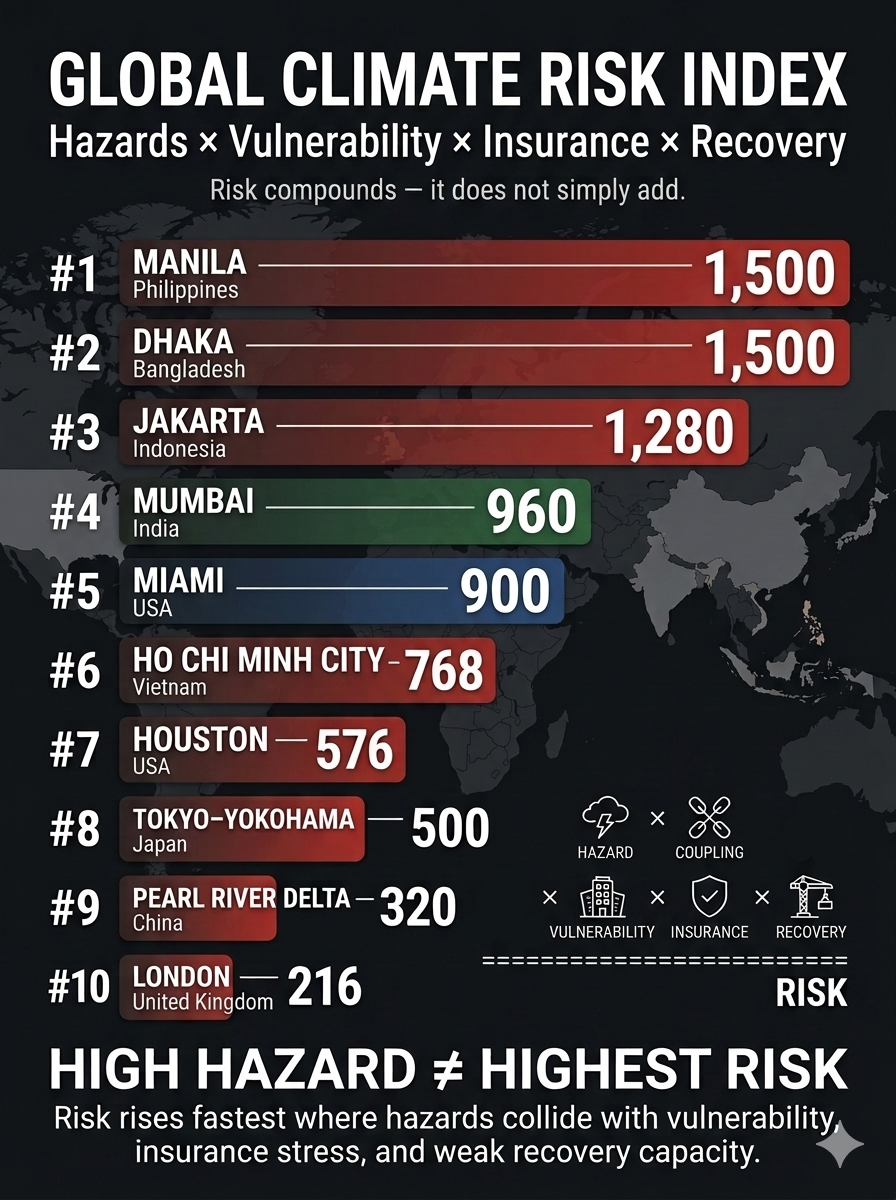
Hazard Exposure × Hazard Coupling × Vulnerability × Insurance Stress × Recovery Deficit = Multiplicative Real Estate Climate Risk

The resulting score is a comparative risk factor rather than a probability of loss or a forecast of future property values.


1. Manila & Central Luzon, Philippines

Hazard Exposure (5): Exceptional exposure to multiple severe Pacific typhoons, coastal storm surge, extreme rainfall, river flooding, and sea-level rise.

Hazard Coupling (5): Storm surge can coincide with torrential rainfall and river flooding, trapping inland water and producing prolonged flooding across low-lying urban districts.

Vulnerability (4): High population density, uneven construction quality, aging structures, and extensive informal development increase exposure to severe wind and flood damage.

Insurance Stress (3): Commercial insurance is more accessible for premium assets than for much of the broader property market, leaving substantial portions of residential and lower-value real estate underinsured.

Recovery Deficit (5): Severe recovery constraints can arise from infrastructure damage, disrupted electrical systems, engineering shortages, and delays in mobilizing reconstruction resources.

Total Multiplicative Risk: 5 × 5 × 4 × 3 × 5 = 1,500


2. Dhaka, Bangladesh

Hazard Exposure (4): Extreme exposure to tropical cyclones, riverine flooding, intense rainfall, extreme heat, and broader regional water stress.

Hazard Coupling (5): Extreme heat, heavy precipitation, drainage limitations, river flooding, and rapidly expanding urbanization can interact to amplify infrastructure and property losses.

Vulnerability (5): Large concentrations of densely developed, lower-quality and non-engineered structures create substantial exposure to flooding, subsidence, and extreme weather.

Insurance Stress (3): Formal property insurance penetration remains limited, leaving many losses concentrated on property owners and investors rather than broadly distributed through insurance markets.

Recovery Deficit (5): Limited fiscal capacity, infrastructure constraints, and dependence on external recovery financing can substantially extend post-disaster reconstruction.

Total Multiplicative Risk: 4 × 5 × 5 × 3 × 5 = 1,500


3. Greater Jakarta Area (Jabodetabek), Indonesia

Hazard Exposure (4): Severe exposure to chronic land subsidence, monsoonal flooding, extreme rainfall, coastal inundation, and sea-level rise.

Hazard Coupling (5): Land subsidence increases the effective impact of rising seas and high tides, while intense rainfall can overwhelm drainage systems and compound coastal flooding.

Vulnerability (4): Dense development, vulnerable transportation and utility infrastructure, and extensive below-grade systems increase exposure to flood-related disruption.

Insurance Stress (4): High climate-related losses and growing flood exposure can increase underwriting pressure, exclusions, deductibles, and affordability challenges.

Recovery Deficit (4): Major infrastructure investments are underway, but the scale of the metropolitan region and continuing subsidence create substantial long-term recovery and adaptation requirements.

Total Multiplicative Risk: 4 × 5 × 4 × 4 × 4 = 1,280


4. Mumbai Metropolitan Region, India

Hazard Exposure (4): High exposure to intense monsoon rainfall, coastal flooding, tropical cyclones, sea-level rise, and extreme heat.

Hazard Coupling (5): Extreme rainfall interacting with dense urbanization, inadequate drainage, coastal flooding, and heat stress can produce cascading infrastructure and real-estate disruption.

Vulnerability (4): Rapid development, extensive reclaimed land, aging buildings, and high-density urbanization increase exposure to flooding, structural deterioration, and infrastructure failure.

Insurance Stress (3): Climate-risk insurance penetration remains uneven, while rising exposure to flood and heat losses places increasing pressure on commercial and residential property coverage.

Recovery Deficit (4): Aging drainage systems, infrastructure deficits, population density, and high emergency-service demands can prolong recovery following major events.

Total Multiplicative Risk: 4 × 5 × 4 × 3 × 4 = 960


5. Miami & Southeast Florida, United States

Hazard Exposure (5): Exceptional exposure to major Atlantic hurricanes, storm surge, sea-level rise, tidal flooding, and recurrent coastal inundation.

Hazard Coupling (4): Storm surge, rainfall, rising seas, groundwater interactions, and porous limestone geology can combine to produce flooding beyond areas directly affected by rainfall.

Vulnerability (3): Modern buildings benefit from increasingly stringent wind standards, but extensive older and mid-tier residential and commercial properties remain vulnerable to wind, flood, and water intrusion.

Insurance Stress (5): Extreme insurance stress is driven by carrier withdrawals, rising premiums, higher deductibles, reinsurance costs, and growing exposure to catastrophic losses.

Recovery Deficit (3): High private wealth, federal disaster resources, and substantial construction capacity support recovery, although repeated disasters can strain public infrastructure and municipal finances.

Total Multiplicative Risk: 5 × 4 × 3 × 5 × 3 = 900


6. Ho Chi Minh City & Mekong Delta, Vietnam

Hazard Exposure (4): High exposure to chronic flooding, tropical storms, sea-level rise, extreme rainfall, and land subsidence.

Hazard Coupling (4): Tidal intrusion, river flooding, subsidence, upstream water management, and intense rainfall can combine to produce prolonged inundation.

Vulnerability (4): Large concentrations of low-rise residential, industrial, and manufacturing properties remain exposed to flooding and often lack comprehensive floodproofing or elevated mechanical systems.

Insurance Stress (3): Industrial assets may have access to international insurance capacity, but climate-risk pricing and coverage remain uneven across the broader real-estate market.

Recovery Deficit (4): Infrastructure investment continues to expand, but rapid urban and industrial growth can outpace drainage, flood-control, and adaptation capacity.

Total Multiplicative Risk: 4 × 4 × 4 × 3 × 4 = 768


7. Houston & Southeast Texas Gulf, United States

Hazard Exposure (4): High exposure to extreme rainfall, hurricanes, storm surge, coastal flooding, and occasional severe winter weather.

Hazard Coupling (4): Intense rainfall interacting with extensive impervious urban surfaces, bayous, drainage limitations, and coastal water levels can generate widespread property inundation.

Vulnerability (3): Large concentrations of slab-on-grade development and extensive construction across flood-prone areas increase exposure to flooding and infrastructure disruption.

Insurance Stress (4): Rising catastrophe losses, increasing deductibles, and elevated wind, hail, and flood costs place substantial financial risk on property owners.

Recovery Deficit (3): Strong corporate and regional financial capacity supports recovery, but large-scale flood-control, grid, and infrastructure projects can require years to complete.

Total Multiplicative Risk: 4 × 4 × 3 × 4 × 3 = 576


8. Tokyo-Yokohama Metropolitan Area, Japan

Hazard Exposure (5): Exceptional exposure to typhoons, storm surge, extreme rainfall, coastal flooding, and major seismic hazards.

Hazard Coupling (5): Typhoon rainfall can saturate soils and simultaneously trigger landslides, flooding, drainage failures, and infrastructure disruptions.

Vulnerability (2): Strong seismic engineering, rigorous building standards, sophisticated infrastructure, and extensive disaster-preparedness systems substantially reduce structural vulnerability.

Insurance Stress (5): Despite strong domestic resilience, the concentration of enormous asset values and catastrophe exposure creates substantial insurance and reinsurance accumulation risk.

Recovery Deficit (2): Strong national institutions, advanced emergency logistics, substantial financial capacity, and sophisticated construction and engineering systems support comparatively rapid recovery.

Total Multiplicative Risk: 5 × 5 × 2 × 5 × 2 = 500


9. Pearl River Delta — Hong Kong, Shenzhen & Guangzhou, China

Hazard Exposure (5): Exceptional exposure to typhoons, extreme precipitation, coastal flooding, sea-level rise, and heat.

Hazard Coupling (4): Extreme rainfall, storm surge, drainage constraints, underground infrastructure, and disruptions to industrial power and supply chains can interact to create cascading losses.

Vulnerability (2): Modern high-rise construction, extensive engineered infrastructure, and substantial flood and coastal defenses reduce the probability of widespread structural failure.

Insurance Stress (4): The extraordinary concentration of commercial and industrial assets creates significant aggregate-loss exposure for insurers and reinsurers during major catastrophes.

Recovery Deficit (2): Strong governmental capacity, extensive infrastructure, rapid mobilization, and substantial financial resources support comparatively rapid physical recovery.

Total Multiplicative Risk: 5 × 4 × 2 × 4 × 2 = 320


10. London & Thames Estuary, United Kingdom

Hazard Exposure (3): Moderate exposure to storm surge, coastal and river flooding, winter storms, extreme rainfall, and increasing heat stress.

Hazard Coupling (4): Sea-level rise increases pressure on tidal defenses, while a major surge combined with heavy rainfall could disrupt transportation, underground infrastructure, and commercial districts simultaneously.

Vulnerability (3): Extensive historic building stock, aging infrastructure, subsidence-sensitive soils, and limited cooling capacity increase exposure to certain climate hazards.

Insurance Stress (3): Insurance remains broadly accessible, but increasing exposure to flooding, heat, subsidence, and other climate-related losses may increase premiums and underwriting constraints.

Recovery Deficit (2): Strong institutions, substantial fiscal capacity, sophisticated infrastructure, and extensive engineering resources provide significant recovery advantages.

Total Multiplicative Risk: 3 × 4 × 3 × 3 × 2 = 216


Global Climate Risk Index Matrix

Because the framework is multiplicative rather than additive, high structural vulnerability and limited recovery capacity can propel a region above a wealthier, more technologically advanced city even when the latter faces greater absolute exposure to extreme weather.

RankGlobal RegionHazard ExposureHazard CouplingVulnerabilityInsurance StressRecovery DeficitMultiplicative Risk
1Manila & Central Luzon, Philippines554351,500
2Dhaka, Bangladesh455351,500
3Greater Jakarta, Indonesia454441,280
4Mumbai, India45434960
5Miami & Southeast Florida, USA54353900
6Ho Chi Minh City & Mekong Delta, Vietnam44434768
7Houston & Southeast Texas Gulf, USA44343576
8Tokyo-Yokohama, Japan55252500
9Pearl River Delta, China54242320
10London & Thames Estuary, UK34332216

What the Multiplicative Model Reveals

The ranking produces an important result: the most dangerous real-estate markets are not necessarily those with the most extreme individual hazards.

The multiplicative structure rewards resilience and penalizes systemic weakness. A highly exposed city with strong building standards, deep financial reserves, robust infrastructure, and rapid recovery capacity can therefore rank below a less technologically advanced city where multiple vulnerabilities interact.

This is the central insight of the model:

Climate risk is not simply where hazards are strongest. It is where hazards, vulnerability, insurance stress, and recovery deficits compound.

The greatest real-estate risks emerge when physical climate exposure becomes financially and institutionally amplified—turning a weather event into a prolonged property, insurance, infrastructure, and investment crisis.

bookmark_borderCoupled Climate Feedbacks and Cascading Real Estate Risk

by Daniel Brouse and Sidd Mukherjee

How Compound Flooding Is Reshaping Property Values, Insurance Availability, and Coastal Habitability

Climate change is creating a new class of real-estate risk in which the physical hazards of flooding increasingly interact with financial, insurance, infrastructure, and housing systems. Sea-level rise, heavier precipitation, and more intense or slower-moving hurricanes are not independent threats. They can interact to produce compound flooding, while the increasing frequency of damaging events can compress the time available for communities, property owners, insurers, and governments to recover.

The consequences extend far beyond the immediate cost of flood damage. As flood frequency increases, historical assumptions about property risk, insurance pricing, mortgage security, infrastructure design, and long-term property values become progressively less reliable. A property that was once considered a low-probability flood risk can become repeatedly exposed to flooding without the physical structure itself changing. As risk is repriced, insurance can become more expensive, less available, or unavailable altogether. Declining insurability can then reduce property values, constrain mortgage lending, discourage investment, weaken local tax bases, and reduce the resources available for infrastructure maintenance and adaptation.

This creates a coupled socioeconomic feedback loop:

Climate Warming → Hazard Intensification → Hazard Coupling → Compound Flooding → Damage and Losses → Insurance Stress → Property-Value Pressure → Reduced Investment → Infrastructure and Resilience Erosion → Greater Vulnerability → Greater Future Losses

A second feedback develops as recovery intervals contract:

Flood Frequency ↑ → Recovery Time Available ↓ → Unresolved Damage ↑ → Vulnerability ↑ → Subsequent Losses ↑

The resulting process is not simply an increase in flood risk. It is a potential transformation of real estate from a relatively stable store of household and institutional wealth into an increasingly climate-sensitive asset whose value, insurability, and financing depend upon the interaction of physical hazards and socioeconomic resilience.

The central argument of this paper is that real estate and insurance may become among the earliest and most visible indicators of cascading climate risk. When insurance becomes unaffordable or unavailable, property values weaken, lenders reassess collateral, investment retreats, and municipalities lose portions of their tax base, the effects of climate change have moved from the physical environment into the financial structure of communities.


1. Introduction: Climate Risk Is Becoming Real-Estate Risk

Climate change is often described in terms of rising temperatures, heavier rainfall, stronger storms, sea-level rise, and increasingly frequent flooding. Yet for households and communities, the most consequential effects may be transmitted through a different system:

Real Estate → Insurance → Mortgage Finance → Investment → Municipal Revenue → Infrastructure → Property Risk

A flood does not have to destroy a property to damage its economic value.

A property can lose value because:

  • flooding becomes more frequent;
  • flood insurance becomes more expensive;
  • insurance coverage becomes difficult to obtain;
  • insurers withdraw from the market;
  • lenders become more cautious;
  • infrastructure becomes less reliable;
  • buyers perceive increasing future risk;
  • investors demand higher returns for greater exposure;
  • municipal finances deteriorate;
  • repeated flooding reduces confidence in long-term habitability.

This changes the nature of climate risk.

The relevant question is no longer simply:

How much physical damage will the next flood cause?

It becomes:

What happens to the economic value and insurability of property when floods repeatedly occur before the community has fully recovered from previous events?

That is a fundamentally different risk problem.


2. Hurricane Harvey: The Beginning of the Feedback Chain

Hurricane Harvey provides a useful illustration of the physical mechanism underlying this emerging financial risk.

In August 2017, Harvey stalled over Texas and produced more than 40 inches of rainfall across a large area. At Nederland, Texas, 60.58 inches of rain was recorded, the largest single rainfall total associated with a tropical cyclone or its remnants in the United States. Damage was estimated at approximately $164 billion in 2026 dollars, with flooding responsible for most of the losses.

Harvey was also a compound-flood event.

Runoff from extreme rainfall moved toward the Gulf while storm surge pushed seawater inland. The elevated coastal water interfered with drainage, producing flooding through the interaction of rainfall runoff and storm surge.

The physical mechanism can therefore be expressed as:

Extreme Rainfall + Runoff + Storm Surge → Drainage Impairment → Compound Flooding

Climate change adds additional forcing:

Climate Warming → Heavier Rainfall + Higher Sea Level + More Intense/Slower Storms → Greater Compound Flood Risk

But the economic cascade begins after the water arrives:

Compound Flooding → Property Damage → Insurance Claims → Insurance Losses → Higher Insurance Costs and Reduced Availability

This is where physical climate risk begins to transform into financial risk.


3. The Three-Way Climate Pressure on Property

Three major mechanisms increasing compound flood risk along the U.S. Atlantic and Gulf coasts:

  1. More intense and slower-moving hurricanes
  2. Increased heavy precipitation as warmer air holds more water vapor
  3. Sea-level rise.

These mechanisms vary geographically.

Across the Gulf of Mexico and Florida, increased rainfall is projected to be the dominant driver in many locations. Across portions of the Southeast and Mid-Atlantic, changes in intense or slow-moving hurricanes become more important. Along the upper Mid-Atlantic and New England coasts, sea-level rise becomes increasingly dominant.

From a real-estate perspective, however, the distinction between the individual drivers may matter less than their combined effect.

The property does not experience three separate balance sheets.

It experiences one risk environment.

The resulting relationship is:

Sea-Level Rise + Extreme Rainfall + Storm Intensification → Compound Flood Risk → Property Risk

The financial system then responds:

Property Risk ↑ → Insurance Risk ↑ → Financing Risk ↑ → Property Value Pressure ↑

This is the beginning of the real-estate cascade.


4. Compound Flooding Creates Nonlinear Property Risk

The Harvey evidence demonstrates why conventional property-risk calculations can become inadequate.

A 2023 study found that approximately 19% of the flood area around Port Arthur, Texas, during Harvey resulted from compound flooding.

Under a scenario involving 0.57 meters of additional sea-level rise and 18% more rainfall, described as plausible around 2050, the compound-flooding area increased to 33%.

Under a scenario involving 1.6 meters of sea-level rise and 50% additional rainfall, described as plausible by 2100, compound flooding increased to 46%, while the number of structures affected was estimated to increase by approximately 23 times compared with 2017.

This is important for property markets because exposure can increase much faster than any single climate variable.

The relevant relationship is:

Climate Forcing ↑ → Hazard Interaction ↑ → Flood Exposure ↑↑ → Property Risk ↑↑

A property market that prices risk based primarily on historical flood frequency may therefore systematically underestimate future exposure.


5. The Return-Period Problem Becomes a Property-Valuation Problem

Real estate depends heavily on expectations about future risk.

A home buyer, mortgage lender, insurer, developer, or investor is effectively making a long-term assessment:

What is the probability that this property will suffer damaging losses during the period in which I own or finance it?

Historically rare floods can become much more frequent as the physical baseline changes.

Research found that human-driven sea-level rise has quadrupled the frequency of coastal sea-level extremes since 1900. At several locations, relative sea-level rise transformed a coastal flood that was a 100-year event in 1900 into an event occurring every five years or less frequently by 2005.

Recent examples illustrate the magnitude of this transformation.

A flood that historically occurred approximately once every ten years occurred:

Charleston → 17 times in 2025

Galveston → 9 times in 2024

Atlantic City → 10 times in 2024

Miami → 14 consecutive days in October 2025

Key West → 26 of 27 days in October 2025

For real estate, this represents a fundamental repricing problem.

A property does not need to be destroyed for its value proposition to change.

If the frequency of disruptive flooding changes from:

Rare → Occasional → Frequent → Persistent

then the economic characteristics of the property can change correspondingly.


6. The Insurance Market Is the First Financial Transmission Mechanism

Insurance is designed to transfer risk.

But insurance markets depend upon the ability to estimate and diversify that risk.

When climate change causes historical loss probabilities to change rapidly, insurers face a fundamental problem:

Historical Risk Models → Changing Climate Baseline → Increasing Loss Uncertainty

The response can take several forms:

Risk ↑ → Premiums ↑

Risk ↑ → Deductibles ↑

Risk ↑ → Coverage Restrictions ↑

Risk ↑ → Capacity ↓

Risk ↑ → Insurer Withdrawal ↑

For individual homeowners, the immediate consequence is affordability.

For the real-estate market, the deeper consequence is insurability.

Insurance availability is not simply another household expense.

It is part of the financial infrastructure supporting property ownership.


7. Insurance Availability Can Become a Property-Value Constraint

A property with affordable insurance can be financed, sold, and occupied relatively normally.

A property with extremely expensive insurance is economically less attractive.

A property that cannot obtain insurance may become difficult to finance.

The chain becomes:

Flood Risk ↑ → Insurance Cost ↑ → Ownership Cost ↑ → Buyer Demand ↓ → Property Value Pressure ↑

But the cascade can become stronger:

Flood Risk ↑ → Insurance Availability ↓ → Mortgage Financing Constraints ↑ → Buyer Pool ↓ → Property Liquidity ↓ → Property Values ↓

This produces a potentially powerful feedback.

As property values decline:

Property Values ↓ → Tax Base ↓ → Municipal Revenue ↓ → Infrastructure Investment Capacity ↓

If infrastructure resilience subsequently deteriorates:

Infrastructure Resilience ↓ → Flood Vulnerability ↑ → Property Risk ↑

The cycle closes:

Property Values ↓ → Tax Base ↓ → Infrastructure Capacity ↓ → Flood Risk ↑ → Insurance Stress ↑ → Property Values ↓

This is a coupled socioeconomic feedback loop.


8. The Insurance–Mortgage–Real Estate Feedback

Insurance and mortgage finance are closely connected.

A mortgage is a long-duration financial claim secured by an asset expected to retain sufficient value to protect the lender.

As flood risk increases, the financial system therefore confronts several interconnected questions:

Can the property be insured?

At what cost?

Will the property retain its value?

Will future buyers be able to obtain financing?

Will the property remain inhabitable?

The resulting feedback can be represented as:

Flood Risk ↑ → Insurance Risk ↑ → Insurance Cost/Availability Deteriorates → Mortgage Risk ↑ → Lending Constraints ↑ → Buyer Demand ↓ → Property Values ↓

The consequences can extend beyond individual homeowners.

Banks and mortgage investors may increasingly need to evaluate climate exposure at the portfolio level.

A geographic concentration of properties exposed to the same flood hazard creates correlated risk.

Unlike independent household losses, a major regional flood can affect thousands or millions of properties simultaneously.

That makes diversification more difficult.


9. Compound Flooding Creates Correlated Insurance Losses

This is one of the most important implications of compound hazards.

Insurance works most effectively when losses are sufficiently diversified.

But compound climate events can create geographically concentrated losses:

Extreme Rainfall + Storm Surge + High Sea Level → Regional Flooding → Thousands of Simultaneous Claims

A major hurricane can therefore produce simultaneous losses across:

  • homes
  • commercial properties
  • vehicles
  • infrastructure
  • businesses
  • utilities
  • municipal facilities

As compound events become more frequent, the financial system can face increasingly correlated losses.

That creates a feedback:

Compound Events ↑ → Correlated Claims ↑ → Insurer Losses ↑ → Pricing Pressure ↑ → Capacity Constraints ↑

This is fundamentally different from a world in which extreme floods are rare and geographically isolated.


10. Return-Period Compression Changes the Insurance Equation

Research examined extreme compound flooding defined as a one-in-100-year storm surge occurring simultaneously with a one-in-100-year rainfall event.

Historically, the combined event had a return period of approximately 200–500 years along the Gulf and southeastern Atlantic coasts and up to 1,000 years or more in parts of New England. Under an extreme warming scenario for 2100, the frequency increased by approximately 7–36 times in the South and 30–195 times farther north.

For insurance markets, the key issue is not the terminology “100-year event.”

The key issue is the frequency of claims-producing events.

If an event once expected to occur once in several centuries begins occurring multiple times within an insurance portfolio’s planning horizon, historical loss assumptions become increasingly unreliable.

Thus:

Return Interval ↓ → Claims Frequency ↑ → Expected Losses ↑ → Premium Pressure ↑ → Insurance Availability ↓


11. Stronger and Slower Hurricanes Increase Insurance Exposure

Our modeling projects the strongest hurricanes could become approximately 15–30% more intense while moving 20–30% more slowly along much of the U.S. coast. The combination increases the probability of simultaneous extreme rainfall and storm tide.

For property markets, this produces multiple simultaneous threats:

Intensity ↑ → Wind Damage ↑

Intensity ↑ → Storm Surge ↑

Intensity ↑ → Rainfall Potential ↑

Translation Speed ↓ → Rainfall Duration ↑

The combined result is:

Stronger + Slower Storms → Wind + Surge + Rainfall → Compound Property Losses

The insurance consequences can therefore be substantially larger than those associated with a simple increase in storm frequency.


12. Inland Property Markets Are Increasingly Exposed

Flood risk is not confined to oceanfront real estate.

Research finds substantial compound-flooding risks farther inland, including along Gulf Coast rivers where high streamflow can interact with storm surge. Increasing evidence suggests compound flooding can be greatest inland near the limit of tidal influence rather than directly at the coast.

A 2026 preprint found substantial increases in the probability of compound wind and precipitation extremes both within 100 kilometers of the coast and 100–500 kilometers inland under an extreme warming projection.

The significance for real estate is considerable.

Flood risk can migrate geographically.

Coastal Risk → Inland Watershed Risk → Inland Property Exposure

Communities that historically considered themselves outside the principal flood-risk zone can increasingly encounter climate-driven flooding.

That creates a major valuation problem because local markets may have little historical experience with these events.


13. Urban Flooding Creates a New Real-Estate Risk

Urban flooding introduces another dimension.

Extreme precipitation can overwhelm drainage systems even where properties are far from coastlines and major rivers.

The risk can become particularly acute in below-grade housing.

Extreme Rainfall → Stormwater System Overload → Rapid Urban Flooding → Basement/Below-Grade Exposure → Life-Safety Risk

This matters to real estate because conventional flood-risk perceptions often emphasize proximity to rivers, coastlines, or mapped floodplains.

But intense rainfall can create dangerous flooding through overwhelmed urban drainage systems.

As a result:

Flood Risk ≠ Coastal Risk Alone

Increasingly:

Flood Risk = Coastal + Riverine + Pluvial + Urban + Compound Risk

This expansion complicates property valuation, insurance underwriting, and municipal planning.


14. Recovery Deficit Is the Hidden Variable

The most important variable in cascading real-estate risk may not be flood magnitude.

It may be recovery time.

Consider:

Flood A → Damage → Partial Recovery → Flood B → Additional Damage → Partial Recovery → Flood C

If each event arrives before full recovery, unresolved losses accumulate.

A conceptual relationship is:

Resilience(t+1) = Resilience(t) + Recovery(t) − Damage(t)

When:

Recovery > Damage → Resilience Restored

But when:

Damage > Recovery → Resilience Declines

This creates a critical threshold:

Damage Rate > Recovery Rate

Once that condition persists, the system enters a recovery deficit.

For real estate, the consequences include:

Unrepaired Properties → Deferred Maintenance → Lower Property Quality → Lower Values → Reduced Investment → Greater Vulnerability

The property market therefore becomes a mechanism through which physical climate shocks can accumulate.


15. Repeated Flooding Can Produce a Negative Wealth Feedback

Homeownership represents a substantial component of household wealth.

Repeated climate-related losses can therefore create a feedback involving household balance sheets.

Flooding ↑ → Repair Costs ↑ → Insurance Costs ↑ → Property Values ↓ → Household Equity ↓ → Financial Resilience ↓

Lower household financial resilience can make recovery more difficult:

Financial Resilience ↓ → Delayed Repairs → Property Condition ↓ → Property Value ↓

The resulting loop becomes:

Flood Risk ↑ → Property Damage ↑ → Household Wealth ↓ → Recovery Capacity ↓ → Property Vulnerability ↑ → Future Losses ↑

This is particularly significant in communities where property represents a large share of household net worth.

Climate risk can therefore become wealth risk.


16. The Municipal Feedback Loop

The consequences do not stop at individual properties.

Municipal governments depend heavily on property values and economic activity.

A potential cascade is:

Flood Frequency ↑ → Property Damage ↑ → Property Values ↓ → Tax Base ↓ → Municipal Revenue ↓

The municipality then has fewer resources available for:

  • drainage improvements
  • flood defenses
  • road repair
  • stormwater systems
  • emergency response
  • public infrastructure maintenance
  • adaptation

This can produce:

Municipal Revenue ↓ → Infrastructure Investment ↓ → Resilience ↓ → Flood Damage ↑

The feedback closes:

Flood Risk ↑ → Property Values ↓ → Tax Base ↓ → Infrastructure Capacity ↓ → Flood Vulnerability ↑ → Property Risk ↑

At this point, the climate hazard has become embedded in the fiscal condition of the community.


17. The Insurance–Property–Infrastructure Feedback

The major feedback loops can be integrated into a single system:

Climate Warming → Hazard Intensification → Hazard Coupling → Compound Flooding → Physical Damage → Insurance Losses → Premiums/Availability Pressure → Property Value Decline → Investment Decline → Tax Base Erosion → Infrastructure Investment Decline → Resilience Erosion → Greater Flood Vulnerability → Greater Future Losses

This is the core cascading-risk mechanism.

The system is not linear.

Each component can alter the conditions affecting the next component.

The physical climate hazard creates the initial disturbance.

The socioeconomic system can then amplify the disturbance.


18. Insurance May Become an Early-Warning System for Climate Risk

Insurance markets have an unusual role in this transition.

They continuously translate physical risk into financial pricing.

Consequently, insurance-market changes may provide an early indicator of emerging real-estate instability.

The sequence may be:

Physical Risk ↑ → Actuarial Risk ↑ → Premiums ↑ → Deductibles ↑ → Coverage Restrictions ↑ → Insurer Withdrawal ↑

These signals can appear before large-scale property abandonment.

A community may therefore be approaching a real-estate resilience threshold even when most houses remain physically intact.

The early warning may instead appear as:

Insurance Availability ↓

Insurance Affordability ↓

Mortgage Availability ↓

Property Transactions ↓

Investment ↓

Property Values ↓

This suggests that insurance markets should be viewed not merely as financial institutions absorbing climate losses, but as risk sensors embedded within the real-estate system.


19. The Property-Value Feedback Can Accelerate

Once buyers begin incorporating future flood risk into property decisions, market expectations can change.

The feedback can become:

Flood Frequency ↑ → Risk Perception ↑ → Buyer Demand ↓ → Property Values ↓

Lower values can then produce additional effects:

Property Values ↓ → Equity ↓ → Investment ↓ → Maintenance ↓ → Vulnerability ↑

And:

Property Values ↓ → Tax Base ↓ → Public Infrastructure Investment ↓ → Vulnerability ↑

And:

Flood Risk ↑ → Insurance Costs ↑ → Total Cost of Ownership ↑ → Buyer Demand ↓ → Property Values ↓

The system therefore contains multiple reinforcing loops operating simultaneously.

This is what distinguishes a coupled-feedback system from a simple hazard-impact model.


20. The Sandy Example: An Accelerating Financial Risk Clock

Research found that a Sandy-like event in New York City, estimated at approximately once every 150 years in the current climate, could become approximately a once-in-65-year event by 2050 and once-in-30-year event by 2100 under the emissions scenario studied.

From a real-estate perspective, the significance is not simply that the probability of flooding increases.

The economic life of a mortgage, insurance policy, or property investment may span decades.

A hazard that occurs once every 150 years has a very different economic significance from one occurring once every 30 years.

Thus:

Return Interval ↓ → Probability of Loss During Ownership ↑ → Insurance Risk ↑ → Mortgage Risk ↑ → Property Risk ↑

The longer the investment horizon, the more consequential the changing hazard frequency becomes.


21. Sea-Level Rise Creates a Persistent Baseline Shift

Sea-level rise differs from many episodic hazards because it permanently alters the starting point from which future storms occur.

A higher ocean means:

Higher Baseline Water Level → Greater Storm-Surge Reach → Greater Flood Exposure

And:

Sea-Level Rise → Less Drainage Capacity → Greater Interaction Between Runoff and Surge

This means that even if a future storm were identical to a historical storm, its consequences could be different because it would occur against a changed physical baseline.

For property markets:

Sea-Level Rise → Persistent Risk Increase → Long-Term Property Exposure ↑

This is particularly important for real estate because buildings and infrastructure have long lifetimes.


22. The Coastal Property Paradox

Coastal property can remain economically attractive even while its physical risk is increasing.

That creates a potential divergence:

Amenity Value ↑

while:

Climate Risk ↑

For a period, rising demand may conceal increasing physical risk.

But eventually the financial system may begin incorporating the changing risk more aggressively.

The transition can be:

Physical Risk ↑ → Insurance Cost ↑ → Ownership Cost ↑ → Market Awareness ↑ → Buyer Demand ↓ → Property Values ↓

The result may be a delayed repricing.

Real estate markets do not necessarily respond immediately to slowly accumulating physical risk.

Insurance markets, however, may respond sooner because they must continually price expected losses.

This creates the possibility that:

Insurance repricing precedes real-estate repricing.


23. When Insurance Becomes Unaffordable, the Market Changes

Insurance affordability is particularly important because homeowners do not experience insurance as an abstract actuarial variable.

They experience it as part of the cost of owning a property.

The relevant relationship is:

Mortgage + Property Tax + Insurance + Maintenance + Expected Climate Losses = Cost of Ownership

If insurance premiums rise dramatically:

Insurance Cost ↑ → Total Cost of Ownership ↑

The property must either:

Price ↓

or:

Buyer Demand ↓

or both.

If insurance becomes unavailable:

Insurance Availability ↓ → Financing Constraints ↑ → Buyer Pool ↓ → Market Liquidity ↓

The property may remain physically valuable, but its economic utility as a financed asset declines.


24. From Insurability to Habitability

Insurance is not the only threshold.

Eventually, repeated flooding can affect whether a community remains economically and physically viable.

At the most susceptible U.S. sites, the odds of a one-in-50-year coastal flood could approximately double every five years under continuing sea-level rise. It also notes that many U.S. coastal engineering systems were designed around return periods of roughly 50–100 years.

As historically rare floods become increasingly frequent, the question changes.

It is no longer:

Can we recover from a flood?

It becomes:

Can we maintain a functioning community between floods?

That is the transition from flood risk to habitability risk.


25. The Real-Estate Resilience Threshold

A useful conceptual threshold is:

Insurance Cost + Expected Flood Losses + Infrastructure Costs > Property’s Economic Value Proposition

When this condition becomes persistent, the property may remain physically habitable while becoming economically unattractive.

A second threshold occurs when:

Damage Rate > Recovery Rate

At that point, the property or community cannot fully restore itself between successive events.

A third threshold may emerge when:

Protection Cost > Property Value / Tax Base / Available Capital

At that point, continued protection may become economically difficult.

These thresholds can interact:

Flood Risk ↑ → Insurance Cost ↑ → Property Value ↓ → Tax Base ↓ → Protection Capacity ↓ → Flood Risk ↑

This is a cascading threshold system.


26. From Property Decline to Retreat

The ultimate consequence need not be sudden abandonment.

A more realistic process may occur gradually:

Flood Frequency ↑ → Insurance Stress ↑ → Property Values Stagnate → Investment Declines → Maintenance Declines → Infrastructure Deteriorates → Insurance Availability Declines Further → Property Values Fall → Population Outmigration ↑

Eventually:

Population Decline → Tax Base Decline → Infrastructure Capacity Decline → Resilience Decline

At some point, adaptation may become economically preferable to continued protection.

This can lead to:

Protection → Adaptation → Managed Retreat → Abandonment

The timing and geographic extent of such transitions will vary considerably by location.

The key point is that the transition can be driven not by a single catastrophic flood but by cumulative climate risk interacting with economic feedbacks.


27. The Complete Coupled-Feedback / Cascading Real-Estate Framework

The emerging system can be represented as:

Warming → Hazard Intensification → Hazard Coupling → Compound Flooding → Damage → Insurance Losses → Insurance Cost/Availability Pressure → Property-Value Pressure → Reduced Investment → Tax-Base Erosion → Infrastructure Resilience Decline → Greater Vulnerability → Greater Future Losses

A second loop operates through recovery:

Flood Frequency ↑ → Recovery Window ↓ → Unresolved Damage ↑ → Resilience ↓ → Vulnerability ↑ → Subsequent Damage ↑ → Recovery Window ↓

A third loop operates through insurance:

Flood Risk ↑ → Expected Losses ↑ → Premiums ↑ / Coverage ↓ → Cost of Ownership ↑ → Buyer Demand ↓ → Property Values ↓ → Insurer/Lender Risk ↑ → Insurance and Financing Constraints ↑

A fourth operates through municipal finance:

Property Values ↓ → Tax Base ↓ → Municipal Revenue ↓ → Infrastructure Investment ↓ → Resilience ↓ → Flood Risk ↑ → Property Values ↓

These feedbacks are interconnected.

Together they create:

Climate Forcing → Physical Hazard Coupling → Financial Amplification → Resilience Erosion → Cascading Real-Estate Risk


28. A New Definition of Climate-Exposed Property Risk

Traditional real-estate risk often focuses on:

Location + Structure + Historical Flood Zone

A future-oriented model must incorporate additional variables:

Flood Frequency

Compound-Hazard Probability

Sea-Level Rise

Extreme Precipitation

Storm Intensity and Translation Speed

Insurance Availability

Insurance Affordability

Mortgage Availability

Infrastructure Resilience

Recovery Capacity

Property-Value Trajectory

Municipal Fiscal Capacity

The risk of a property is therefore not simply its probability of flooding.

A more comprehensive conceptual formulation is:

Real-Estate Climate Risk ∝ Hazard Exposure × Hazard Coupling × Vulnerability × Insurance Stress × Recovery Deficit

Again, this is a conceptual framework rather than a validated predictive equation.

Its purpose is to recognize that physical exposure and financial vulnerability can amplify one another.


29. Why Historical Property Valuation Models May Become Increasingly Unreliable

A property valuation based heavily on historical comparable sales assumes that the past provides meaningful information about future risk.

But if the climate baseline is changing:

Historical Flood Frequency ≠ Future Flood Frequency

And therefore:

Historical Property Risk ≠ Future Property Risk

This creates the potential for a valuation lag.

A property may continue selling at prices based on historical assumptions even as:

Flood Frequency ↑

Insurance Cost ↑

Infrastructure Stress ↑

Future Risk ↑

The market can therefore experience a delayed repricing once these factors become visible to buyers, lenders, and insurers.

The longer the delay, the greater the possibility of a discontinuous adjustment.


30. The Central Role of Insurance in Price Discovery

Insurance markets can force climate risk into property economics because they must continually reassess expected losses.

This creates a potentially important sequence:

Physical Climate Change → Insurance Repricing → Mortgage Reassessment → Buyer Reassessment → Property Repricing

In this framework, insurance functions as an intermediary between the climate system and the real-estate market.

This makes insurance availability and affordability among the most important indicators to monitor.

A deteriorating insurance market can signal that the physical risk has become financially material even before large-scale property abandonment occurs.


31. The Emerging Climate-Real-Estate Feedback

The broader system can therefore be summarized as:

Physical System

Warming → Sea-Level Rise + Heavier Rainfall + Stronger/Slower Storms → Compound Flooding

Insurance System

Compound Flooding → Claims → Losses → Premium Increases + Coverage Restrictions + Reduced Capacity

Real-Estate System

Insurance Stress → Cost of Ownership ↑ → Buyer Demand ↓ → Property Values ↓

Financial System

Property Values ↓ → Mortgage Risk ↑ → Lending Constraints ↑ → Investment ↓

Municipal System

Property Values ↓ → Tax Base ↓ → Infrastructure Investment ↓

Resilience System

Infrastructure Investment ↓ → Flood Vulnerability ↑

The loop closes:

Flood Vulnerability ↑ → Compound Flood Risk ↑

This is a coupled climate-financial feedback loop.


32. The Difference Between a Disaster and a Cascading Risk

A conventional disaster model begins and ends with the event:

Storm → Flood → Damage → Recovery

The cascading-risk model is different:

Storm → Compound Flood → Damage → Insurance Loss → Financial Stress → Property-Value Decline → Tax-Base Erosion → Infrastructure Stress → Reduced Resilience → Greater Vulnerability → Next Flood → Greater Damage

The disaster is therefore no longer an isolated event.

It becomes a state-changing event.

Each major flood can alter the economic and physical conditions under which the next flood occurs.

This makes the system path dependent.


33. The Most Important Variable May Be the Time Between Disasters

“The Floods of the Future Won’t Come One at a Time”—captures the central problem.

The issue is not simply that flood events become more severe.

It is that the interval between them can become shorter.

The resulting relationship is:

Flood Frequency ↑ + Recovery Time Constant → Recovery Window ↓

Then:

Recovery Window ↓ + Damage Per Event ↑ → Recovery Deficit ↑

Then:

Recovery Deficit ↑ → Property Condition ↓ + Infrastructure Condition ↓ + Financial Resilience ↓

Then:

Resilience ↓ → Consequences of the Next Flood ↑

This is the mechanism through which frequency becomes amplification.


34. From Compound Flooding to Cascading Real-Estate Instability

The complete process can now be expressed in one horizontal chain:

Warming → Hazard Intensification → Hazard Coupling → Compound Flooding → More Frequent Losses → Insurance Stress → Higher Cost of Ownership → Reduced Buyer Demand → Property-Value Decline → Mortgage and Investment Stress → Tax-Base Erosion → Infrastructure Resilience Decline → Recovery Deficit → Greater Future Flood Vulnerability → Cascading Real-Estate Instability

This is the central thesis of the paper.

The most important climate consequence for real estate may not be the destruction of individual properties.

It may be the progressive deterioration of the economic conditions that make those properties insurable, financeable, maintainable, and desirable.


35. Conclusion: When Climate Risk Becomes Property Risk

The emerging flood threat is fundamentally different from the historical model of isolated disasters.

Climate change is increasing the potential for:

Sea-Level Rise + Heavy Rainfall + Stronger/Slower Hurricanes → Compound Flooding

At the same time:

Flood Frequency ↑ → Recovery Windows ↓

These physical changes increasingly interact with:

Insurance

Mortgage Finance

Property Markets

Municipal Finance

Infrastructure

Household Wealth

The resulting system can develop reinforcing feedbacks:

Flood Risk ↑ → Insurance Stress ↑ → Property Values ↓ → Investment ↓ → Infrastructure Resilience ↓ → Flood Vulnerability ↑

and:

Flood Frequency ↑ → Recovery Deficit ↑ → Resilience ↓ → Future Losses ↑

These feedbacks create the possibility of nonlinear and cascading consequences.

The immediate manifestation may be rising insurance premiums, shrinking insurance availability, higher deductibles, declining property demand, or increasing difficulty obtaining mortgages.

The next stage may be declining property values and reduced investment.

The subsequent stage may involve weakening municipal tax bases, deteriorating infrastructure, and increasing difficulty financing adaptation.

The final stage in the most vulnerable locations could involve managed retreat, population displacement, and abandonment.

The critical transition is therefore:

Climate Risk → Insurance Risk → Real-Estate Risk → Financial Risk → Municipal Risk → Resilience Risk → Cascading Systemic Risk

This suggests that real estate and insurance markets should be treated as critical components of the climate system’s socioeconomic response.

Insurance is not merely a mechanism for paying claims after a disaster. It is a mechanism for translating physical risk into financial information.

Real estate is not merely a collection of buildings. It is a store of household wealth, collateral for debt, a source of municipal revenue, and the foundation of local economic activity.

When the physical climate changes, these interconnected systems change with it.

The most consequential question is therefore not simply:

Will a property flood?

It is:

Will the property remain insurable, financeable, valuable, maintainable, and economically viable as the probability of flooding changes?

That is the central real-estate question of the emerging climate era.

The ultimate risk is not a single catastrophic flood.

It is the transition from:

Rare Disaster → Recurrent Hazard → Compound Flooding → Insurance Stress → Property Repricing → Investment Retreat → Resilience Erosion → Cascading Real-Estate Risk

When floods begin arriving faster than properties, infrastructure, insurers, lenders, governments, and communities can adapt, the flood itself becomes only the initiating event.

The deeper crisis is the progressive erosion of the economic and institutional systems that allow a place to remain habitable and investable.

In that sense, the future of climate-exposed real estate may be determined less by whether a property floods once than by whether the surrounding system can continue to recover between floods.

The flood becomes the trigger.
Insurance becomes the transmission mechanism.
Real estate becomes the financial amplifier.
Resilience becomes the limiting factor.
And cascading risk becomes the ultimate consequence.