bookmark_borderEarth’s Energy Imbalance: The Climate System Out of Balance

by Daniel Brouse

Simplified Introduction

🌎 Earth’s Energy Imbalance

Climate change can be understood in one deceptively simple equation:

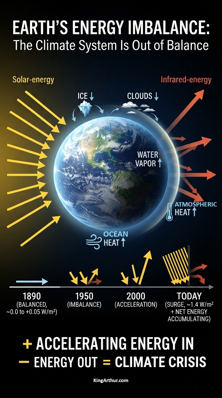
ENERGY IN − ENERGY OUT = ENERGY ACCUMULATING

Earth has been accumulating excess energy for decades. Most of that excess heat—roughly 90%—is going into the oceans.

What matters now is not just that Earth is out of balance, but that the imbalance itself is changing.

The recent acceleration in Earth’s energy imbalance raises an important question:

Are we moving from a relatively steady warming system toward a climate system increasingly driven by interacting feedbacks?

Ice loss. Clouds. Water vapor. Ocean heat. Carbon sinks.

When these systems interact, the climate response can become increasingly nonlinear.

ACCELERATING ENERGY IMBALANCE = ACCELERATING CLIMATE CHANGE

The simplest way to understand global warming may be to stop looking only at the thermometer—and start looking at the energy.

Read the full paper:

The Energy Imbalance (EEI)

A simple way to understand climate change and global warming is through Earth’s energy balance—or, more precisely, the growing lack of balance known as Earth’s Energy Imbalance (EEI).

Earth’s climate is governed by a fundamental exchange: energy arrives primarily from the Sun, while Earth returns energy to space as reflected sunlight and outgoing infrared radiation. When incoming and outgoing energy are equal over the long term, the planet is approximately in energy balance. When more energy enters the Earth system than leaves it, the difference is stored within the climate system, producing warming.

The Basic Energy Equation

There are two fundamental pathways involved in Earth’s energy budget:

  1. Energy enters and leaves.
    Sunlight brings energy into the Earth system, while reflected sunlight and outgoing infrared radiation carry energy back into space.
  2. Energy enters and is temporarily stored.
    Some of the incoming energy remains within the Earth system as heat. It warms the oceans, land, and atmosphere and melts snow and ice. Today, roughly 90% of the excess energy associated with the imbalance is stored in the ocean.

The important point is that energy cannot simply disappear. If less energy leaves the Earth system than enters it, the difference accumulates somewhere within the system.

From Balance to Imbalance

For thousands of years before large-scale industrialization, Earth’s climate system fluctuated around a long-term energy balance. Beginning with the Industrial Revolution, however, human activities increasingly altered that balance.

The primary driver is the buildup of greenhouse gases such as carbon dioxide and methane. These gases reduce the rate at which Earth can emit infrared energy to space. As a result, more energy remains in the Earth system.

This does not mean that every year must be warmer than the preceding year. Natural variability—including El Niño and La Niña—can temporarily redistribute energy between the ocean and atmosphere and produce substantial year-to-year fluctuations. But over longer periods, a persistent positive EEI means that the Earth system continues accumulating energy.

The Imbalance Is Increasing

The remarkable development is not simply that Earth has a positive energy imbalance. The rate of energy accumulation has increased.

NASA and NOAA observations combining CERES satellite measurements with ocean observations found that Earth’s energy imbalance approximately doubled between the first decade of the 21st century and the 2005–2019 period. A 2024 observational assessment likewise found that CERES measured an increase from approximately 0.5 ± 0.2 W/m² during 2000–2009 to 1.0 ± 0.2 W/m² during 2010–2019.

The increase was not simply a matter of more greenhouse gases trapping infrared radiation. The CERES analysis found that absorbed solar radiation increased by about 0.9 W/m², while outgoing longwave radiation increased by about 0.4 W/m², partially offsetting that additional absorbed solar energy.

That distinction is important.

The Earth system can become more energetically unbalanced through changes in both:

  • how much solar energy is absorbed, and
  • how much infrared energy escapes to space.

Why the Post-2020 Period Matters

The years since 2020 have attracted particular scientific attention because several factors have combined to produce unusually large changes in Earth’s radiation budget.

One important contributor is the sharp reduction in sulfur emissions from international shipping following the IMO 2020 regulations. Sulfate aerosols reflect sunlight and can brighten clouds, producing a cooling influence. Their reduction therefore allows more solar radiation to reach and remain within the Earth system.

A 2024 modeling study estimated a global effective radiative forcing from IMO 2020 of approximately +0.14 W/m², primarily through aerosol-cloud interactions. The study estimated that the regulation could contribute about 0.046°C of additional global warming during 2020–2029, while emphasizing that other factors are required to explain the exceptional warmth of 2023.

This is significant, but it should not be interpreted as meaning that shipping regulations alone caused the recent surge in Earth’s energy imbalance.

The climate system is responding simultaneously to greenhouse-gas forcing, aerosol changes, clouds, water vapor, surface albedo, ocean circulation, volcanic activity, and internal variability.

A Rapidly Changing Radiation Budget

CERES observations provide direct measurements of changes in Earth’s radiation budget from space. The data show substantial changes in both absorbed solar radiation and outgoing longwave radiation.

The year 2023 was particularly unusual. Global annual mean absorbed solar radiation was about 1.75 W/m² above the CERES reference climatology, while outgoing longwave radiation was about 0.85 W/m² above the reference. The resulting annual mean net radiation anomaly was approximately +0.90 W/m².

NASA has also reported that 2023 produced exceptionally large anomalies in absorbed solar radiation, with values exceeding the 90% confidence interval for much of March through September. The exceptionally large absorbed-solar and outgoing-longwave anomalies continued into early 2024.

These observations demonstrate something important:

Earth’s energy budget is not static. It is changing.

And the changes involve multiple interacting components of the climate system.

Energy Imbalance and Climate Feedbacks

This is where the concept of climate feedback becomes important.

An initial warming can trigger changes that alter the amount of energy entering or leaving the Earth system. Some of those changes amplify the original warming.

Examples include:

  • Water vapor: Warmer air can hold more water vapor, and water vapor is itself a greenhouse gas.
  • Ice and snow: Melting reduces Earth’s reflectivity, allowing more sunlight to be absorbed.
  • Clouds: Changes in cloud amount, altitude, composition, and properties can alter both reflected sunlight and outgoing infrared radiation.
  • Ocean warming: The ocean absorbs most of the excess energy, affecting circulation, evaporation, sea level, and atmospheric processes.
  • Carbon-cycle feedbacks: Warming and changing environmental conditions can alter the ability of terrestrial and oceanic systems to absorb carbon.

These feedbacks do not create energy from nothing. Rather, they change the pathways through which energy moves through the Earth system.

That distinction is crucial.

A feedback can cause the Earth to absorb more solar energy or retain more infrared energy, increasing the rate at which the existing energy imbalance grows.

The Energy Accumulation Is Enormous

The units used to measure EEI—watts per square meter—can make the imbalance sound deceptively small.

For example, 1.0 W/m² means that, averaged across the entire surface of Earth, approximately one additional joule of energy is accumulating every second for every square meter.

Across the entire planet, even a 1.0 W/m² imbalance corresponds to roughly 510 terawatts of continuous power.

At an imbalance of 1.45 W/m², the corresponding rate would be roughly 740 terawatts.

That is an extraordinary amount of energy.

The comparison can be expressed another way. Using the approximate energy yield of the Hiroshima bomb, an EEI of 1.45 W/m² corresponds to an energy accumulation rate on the order of 11 Hiroshima-scale explosions every second.

The important point is not the metaphor itself. It is the scale of the energy involved.

The Earth Is Not Just Getting Warmer

Temperature is only one visible consequence of the energy imbalance.

The accumulated energy is distributed throughout the Earth system. It:

  • heats the oceans,
  • warms the land,
  • warms the atmosphere,
  • melts glaciers and ice sheets,
  • reduces sea ice,
  • expands seawater,
  • increases evaporation,
  • intensifies the hydrological cycle,
  • and contributes to changes throughout the climate system.

NASA’s CERES program estimates that about 93% of the current excess energy is stored in the ocean, illustrating why ocean heat content is such an important measure of Earth’s changing energy budget.

This is why looking only at surface temperature can obscure part of the story.

The climate system is an energy system.

Surface temperature is one measurement of that system—not the system itself.

The EEI Timeline

Historical Period / EraApproximate EEI Average (W/m²)Primary Radiative Drivers & Climate Context
1890–1910
(Early Industrialization)
~0.0 to +0.05The climate remains in near-equilibrium. Early fossil fuel emissions are largely offset by natural variability and background volcanic activity.
1910–1950
(Mid-Century Rise)
+0.05 to +0.15EEI begins a slight upward crawl. A steady expansion of global manufacturing and coal combustion begins trapping marginal longwave heat.
1950–1970
(The Aerosol Masking Era)
+0.15 to +0.25The “Great Acceleration” of industry begins. However, heavy sulfur dioxide pollution creates a reflective aerosol blanket, blocking sunlight and masking up to half of greenhouse warming.
1970–1990
(Emerging Imbalance)
+0.30 to +0.50Clean air regulations reduce sulfur pollution while greenhouse gases continue to climb. The planet begins absorbing noticeably more solar radiation.
1990–2005
(Systemic Multi-Decade Warming)
+0.50 to +0.65Satellite programs launch. Except for a brief drop following the 1991 Mount Pinatubo volcanic eruption, the EEI remains locked in a consistently positive, warming state.
2005–2019
(The First Acceleration)
+0.70 to +0.90The long-term EEI average effectively doubles compared to prior decades. Ocean heat content spikes dramatically as the oceans absorb roughly 90% of this excess energy.
2020–2023
(The Post-2020 Surge)
+1.00 to +1.30Slashed marine shipping pollution (IMO 2020 regulations) rapidly clears atmospheric haze over the oceans, forcing a massive, sudden spike in absorbed solar energy.
2024–Present
(Nonlinear Feedback Phase)
+1.40 to +1.48+EEI hits unprecedented, record-breaking territory. Strong climate feedbacks—such as collapsing Antarctic sea ice and thinning cloud decks—darken the planet, causing it to absorb immense amounts of solar radiation.

Near balance → emerging imbalance → acceleration → post-2020 surge → nonlinear feedback phase

The observational record therefore supports a clear long-term conclusion: Earth’s energy imbalance has increased substantially over recent decades.

The precise attribution of the most recent changes remains an active area of research.

The Bigger Picture

The simplest way to understand global warming is not to begin with a thermometer.

Begin with energy.

Earth receives energy from the Sun. Earth emits energy back into space. Greenhouse gases, clouds, aerosols, ice, water vapor, and other components of the climate system influence how much energy enters, how much leaves, and how quickly the system responds.

When the equation is balanced, Earth’s average climate can remain relatively stable.

When the equation is persistently unbalanced, energy accumulates.

And when the rate of that accumulation changes, the climate system changes with it.

Global warming is therefore not merely a temperature problem. It is an energy-accounting problem.

The central question is simple:

How much energy is entering the Earth system, how much is leaving, and how rapidly is the difference changing?

That difference is Earth’s Energy Imbalance.

And it is one of the most fundamental measurements of a changing climate.
bookmark_borderHow Is Climate Energy Hitting You? Indonesia: Still Burning

by Daniel Brouse

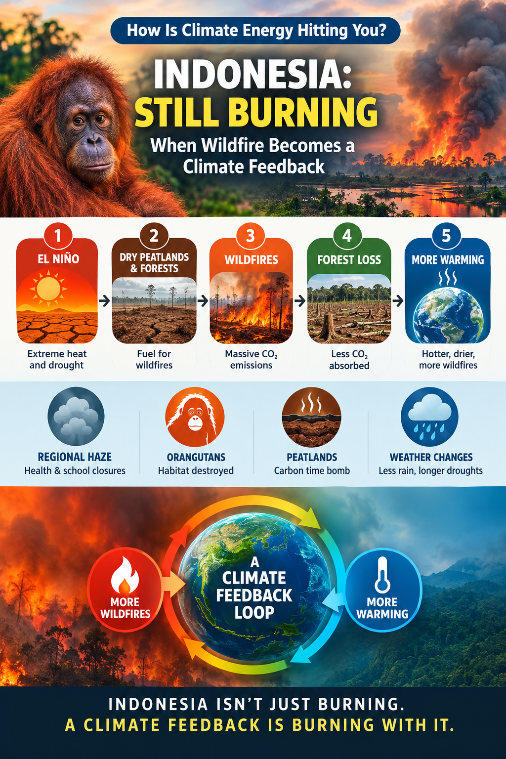
Indonesia: Still Burning — When Wildfire Becomes a Climate Feedback

Indonesia’s wildfire carbon dioxide emissions surged to the highest level in the world in early September 2026, driven by an intense El Niño season and extreme drought.

As reported earlier this month, Indonesia is experiencing a dangerous convergence of climate stress: extreme drought, human land-use change, and increasingly intense wildfires across Sumatra and Borneo.

See: https://www.kingarthur.com/global_warming/Climate-Energy-Orangutans.html

Record Emissions

According to the EU’s Copernicus Atmosphere Monitoring Service, as reported through Fire Emissions Watch, Indonesian fires released approximately 19.7 million metric tons of CO₂ between September 1 and September 7, 2026.

That represented more than one-third of global wildfire CO₂ emissions during that period and surpassed Russia.

The significance goes beyond the immediate emissions. Indonesia contains some of the world’s largest tropical peatlands—vast stores of carbon accumulated over thousands of years. When these peatlands dry out and burn, they can release carbon that has been locked away for centuries or millennia.

Regional Haze and Health Impacts

The consequences are not confined to the fire zones.

Smoke haze has spread across neighboring countries, including Singapore, Malaysia, and the Philippines, producing hazardous air-quality conditions. The resulting disruption has included school closures, remote learning affecting more than a million students, and widespread air-quality warnings.

What begins as a regional wildfire can therefore become a regional atmospheric event—with consequences for human health, transportation, education, agriculture, and ecosystems.

Orangutans Under Threat

Critically endangered orangutans are also facing an escalating survival crisis.

Intense wildfires are destroying and fragmenting habitat across Borneo and Sumatra. Extreme drought makes forests and peatlands more vulnerable to ignition, while the combination of drought, land-use change, and El Niño conditions can transform individual fires into large-scale ecological disasters.

For orangutans, the loss is not simply the burning of individual trees. It is the destruction and fragmentation of an already limited habitat.

When Wildfire Becomes a Climate Feedback

The Indonesian fires illustrate a dangerous climate feedback loop: warming and climate variability can create conditions that produce more wildfire, while the resulting fires release additional greenhouse gases and destroy carbon-absorbing ecosystems.

In other words:

Warming → drought → wildfire → CO₂ release + carbon-sink loss → more warming

Indonesia’s tropical peatlands make this feedback particularly important.

1. The Peatland Carbon Bomb

The process:

Peatlands consist of thick, waterlogged layers of partially decomposed plant material. Because decomposition is slowed under waterlogged conditions, enormous quantities of carbon can accumulate over long periods.

During severe drought, such as that associated with strong El Niño conditions, water tables can fall and peat can dry out.

The feedback:

Once dry, peat can ignite and continue smoldering underground. Unlike an ordinary surface forest fire, a peat fire can persist beneath the surface and release enormous quantities of stored carbon.

That produces a potentially powerful feedback:

Drought → dried peat → peat fire → CO₂ release → increased atmospheric warming → greater drought risk → more peat vulnerability

The critical point is that peat fires can release not only carbon from recently grown vegetation but also carbon accumulated over much longer periods.

2. Destruction of the Rainforest Carbon Sink

The process:

Healthy tropical forests function as major carbon sinks. Through photosynthesis, trees and other vegetation remove CO₂ from the atmosphere and store carbon in biomass and soils.

The feedback:

Wildfire can kill trees, degrade soils, and fragment the forest canopy. The loss of living vegetation reduces the ecosystem’s capacity to remove atmospheric CO₂.

At the same time, dead and damaged vegetation decomposes or burns, returning additional carbon to the atmosphere.

A forest that once removed carbon from the atmosphere can therefore become a source of greenhouse-gas emissions following severe disturbance.

The feedback becomes:

Forest loss → reduced CO₂ uptake + additional emissions → higher atmospheric CO₂ → greater warming

This is a critical distinction: wildfire does not merely add emissions. It can simultaneously remove part of the natural system that would otherwise absorb those emissions.

3. Regional Weather and Surface-Albedo Changes

Wildfires can also modify the physical environment.

Dense smoke and aerosol plumes can spread across enormous areas, reducing incoming sunlight at the surface while altering atmospheric heating. Meanwhile, burned landscapes have different surface characteristics from intact forests, including changes in surface reflectivity, vegetation, soil moisture, and evaporation.

These changes can disrupt local and regional energy and water cycles.

The resulting effects are complex and can vary with atmospheric conditions, but prolonged smoke and vegetation loss can alter evaporation, convection, rainfall patterns, and the persistence of dry conditions.

When drought delays the return of heavy rainfall, peat fires can continue burning underground for extended periods.

The Climate Feedback Loop

The Indonesian situation can be summarized as a sequence:

StepActionImpact
1. TriggerEl Niño + climate warmingIncreased heat and drought stress
2. AmplificationPeatlands and forests dry outLandscapes become increasingly fire-prone
3. EventPeatlands and forests burnLarge quantities of stored carbon are released
4. Carbon-sink lossForests are damaged or destroyedLess CO₂ is removed from the atmosphere
5. Atmospheric responseCO₂ and other greenhouse gases increaseAdditional radiative forcing
6. FeedbackIncreased warming and ecosystem stressGreater risk of future drought and wildfire

The Bigger Picture

The Indonesian fires demonstrate why climate change cannot be understood solely as a gradual increase in average temperature.

Climate energy moves through interconnected Earth systems.

A period of extreme heat and drought can trigger wildfire. Wildfire can release stored carbon. The same wildfire can destroy vegetation that would otherwise absorb atmospheric CO₂. Smoke and land-surface changes can alter regional energy and water cycles. The resulting environmental changes can increase the vulnerability of the system to the next extreme event.

That is a feedback.

And when multiple feedbacks begin operating simultaneously, the climate system can become increasingly difficult to treat as a simple linear progression.

Indonesia isn’t just burning.

A climate feedback is burning with it.

bookmark_borderOil Shipping Costs Explode: From ~$16,000 to More Than $1.2 Million a Day

The cost of transporting crude oil by the world’s largest oil tankers has reached extraordinary levels.

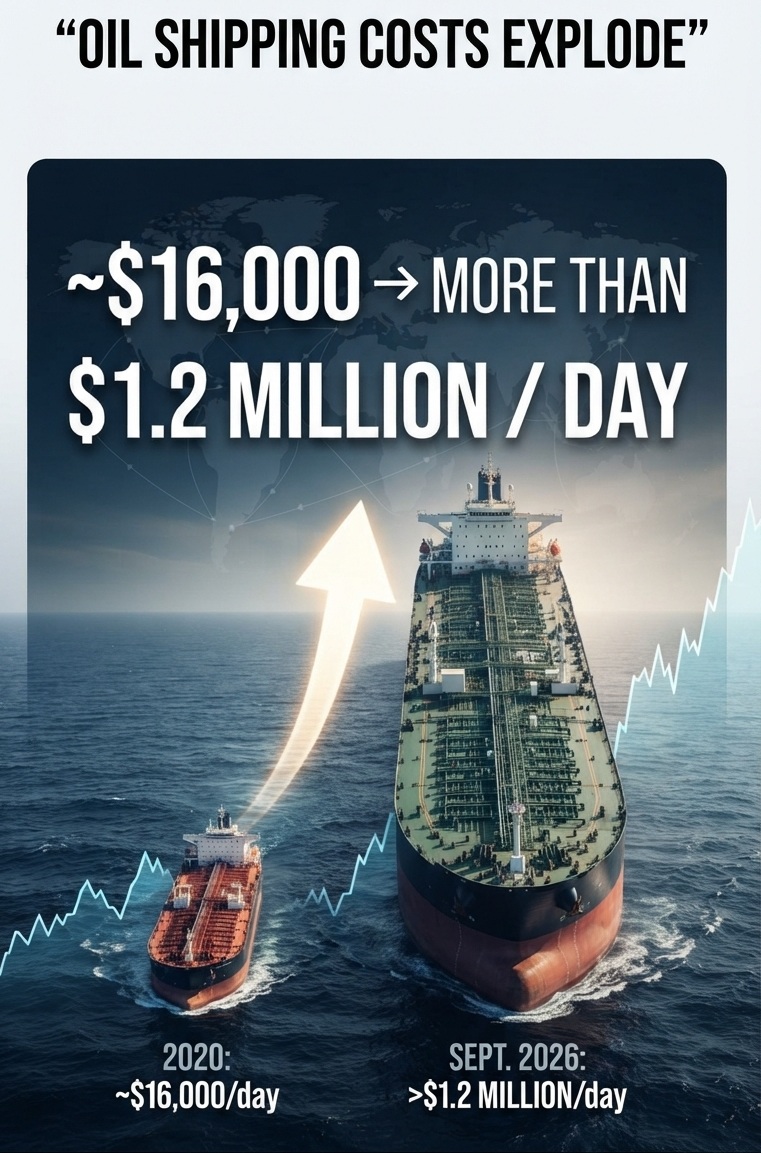
On the benchmark TD3C route — a 270,000-metric-ton Very Large Crude Carrier (VLCC) traveling from the Middle East Gulf to China — daily time-charter-equivalent (TCE) earnings have surged from roughly $16,000/day in 2020 to more than $1.2 million/day in September 2026.

That is not simply a large increase. It represents an extraordinary transformation in the economics of moving oil by sea.

From $16,000 to $1.2 Million a Day

PeriodApprox. TD3C Daily Rate/TCEWhat Was Driving the Market
2020~$16,000/dayPandemic-era demand collapse and abundant tanker capacity
2025~$35,000/day average*Tightening tanker fundamentals, geopolitical rerouting and limited fleet growth
September 2026$1,212,503/dayMiddle East conflict, disruption around the Strait of Hormuz, rerouting and severe tanker scarcity

*McQuilling reported a TD3C average earning of approximately $35,136/day for the first eight months of 2025, rather than $160,000/day.

The 2020 figure is also consistent with contemporary tanker-market estimates. McQuilling projected the TD3C round-trip voyage at approximately $16,200/day for 2020.

Then came 2026.

The $1.2 Million-a-Day Shock

In September 2026, the TD3C benchmark moved into territory rarely seen in modern tanker shipping.

The Baltic Exchange reported that the TD3C rate rose to Worldscale 1,140, corresponding to a round-trip TCE of approximately $1,212,503 per day for a standard Baltic VLCC.

Earlier in September, the same benchmark had already exceeded $1 million/day, with the Baltic assessment reaching approximately $1.099 million/day on September 15.

The surge reflects an extraordinary combination of factors:

  • disruption to Middle Eastern oil-export routes;
  • sharply reduced traffic through the Strait of Hormuz;
  • attacks and security risks affecting regional shipping;
  • longer and more complicated voyages;
  • ships being tied up in shuttle and ship-to-ship operations;
  • and a limited number of immediately available VLCCs.

Reuters reported on September 21 that only 17 commodity vessels transited the Strait of Hormuz over the weekend, compared with 37 the previous week and a pre-conflict average of about 125 vessels per day.

Why Shipping Costs Matter

Oil does not simply move from the wellhead to the refinery.

It has to be transported.

When the cost of transporting a cargo of crude suddenly multiplies, the consequences extend through the entire energy system.

At today’s extreme tanker rates, transportation itself can represent a substantial portion of the delivered cost of crude. The Wall Street Journal reported that VLCC charter costs had exceeded $1 million/day, equivalent to roughly $26 per barrel on the affected voyages.

That means the disruption is not merely a problem for shipowners and oil traders.

It can affect:

oil producers → tanker operators → refiners → fuel distributors → consumers

Higher transportation costs can therefore add pressure to gasoline, diesel, jet fuel and other petroleum products even when the underlying price of crude oil is moving differently.

An Extraordinary Comparison

The scale of the change is easier to see this way:

2020: ~$16,000/day
↓
2025: ~$35,000/day average
↓
September 2026: $1,212,503/day

From the approximate 2020 level to the September 2026 TD3C assessment, the daily TCE increased by roughly 75×.

That is an extraordinary change in the economics of moving a single cargo of oil.

And it demonstrates something important about modern energy systems:

When a critical transportation chokepoint is disrupted, the cost of moving energy can become a crisis of its own.

A market under extreme stress

The current rate should not be interpreted as a normal annual shipping cost. It is a spot-market benchmark during an exceptional geopolitical disruption. Rates can move dramatically in either direction as vessel availability, security conditions, oil flows and trade routes change.

But the magnitude of the September 2026 spike is unmistakable.

The cost of moving oil by VLCC has gone from tens of thousands of dollars per day to more than $1.2 million per day.

That is a remarkable indicator of just how much stress has entered the global oil-transportation system.

bookmark_borderPlug-And-Play Solar

Plug-and-play solar is becoming available around the world—and it could make solar power dramatically simpler and more accessible.

Plug-and-play solar is part of the emerging clean energy economy. Unlike conventional rooftop solar, these small systems can be installed with minimal equipment and, where permitted, connected directly to an existing electrical outlet. That makes solar potentially accessible to renters, apartment dwellers, condominium owners, and homeowners who cannot install a conventional rooftop system.

Cheaper and Healthier

Plug-and-play solar can reduce electricity costs because sunlight is free and the system produces electricity without ongoing fuel purchases. It also generates electricity without the combustion-related air pollutants produced by fossil-fuel power generation.

Instead of buying fuel from a utility to generate electricity somewhere else, a plug-in solar system can capture sunlight right from a balcony, patio, yard, or other suitable location and produce electricity at the point of use.

The basic idea is remarkably simple:

Sunlight → Solar panel → Inverter → Household outlet → Electricity

Great Britain Opens the Door

Great Britain has taken a major step toward making plug-in solar widely accessible. Beginning August 27, 2026, new rules established a legal framework for plug-in solar panels and other plug-in microgenerators.

Under the new framework, qualifying certified systems can connect to standard 13-amp domestic sockets, subject to safety requirements and output limits. Plug-in solar kits can produce up to 800 watts, and users must notify the local electricity network operator. The UK government says the systems could save households up to £110 per year and provide as much as 20% of average household electricity use.

Ofgem has also approved changes to the distribution code intended to facilitate plug-in solar while maintaining requirements for network safety, supply quality, and system operability.

The United States Is Moving State by State

The situation in the United States is less straightforward. There is currently no single nationwide legal framework for plug-in solar. Instead, states are beginning to establish their own rules.

As of September 2026, nine states have enacted legislation specifically addressing plug-in or balcony solar: Utah, Colorado, Maryland, Maine, Vermont, Connecticut, New Hampshire, Virginia, and New Jersey.

Meanwhile, additional states are considering plug-in-solar legislation. California and New York, among others, have active legislative efforts, illustrating how quickly the regulatory landscape is changing.

Plug-and-play solar is therefore more than another solar product. It represents a shift toward small, distributed, consumer-installed energy generation—putting a small power plant within reach of people who may never own a house with a conventional solar roof.

The sun is already there. Plug-and-play solar makes it easier to use.

☀️ THE CLEAN ENERGY ECONOMY

Harmony Hare says:

🔌 PLUG-AND-PLAY SOLAR IS CHEAPER AND HEALTHIER

Solar power doesn’t have to mean a massive rooftop installation.

Plug-and-play solar is changing the equation.

A small solar system can plug directly into an existing electrical outlet—turning a balcony, patio, yard, or other sunny space into a source of clean electricity.

☀️ FREE FUEL
The sun provides the energy. No gasoline. No coal. No natural gas. No ongoing fuel purchases.

💰 LOWER ENERGY COSTS
Generate some of your own electricity instead of buying all of it from the utility.

🌱 CLEANER AIR
Solar electricity generates power without the combustion emissions associated with fossil-fuel generation.

🏠 MORE ACCESSIBLE
Plug-and-play systems can potentially bring solar to renters, apartment dwellers, condo owners, and homeowners who cannot install conventional rooftop solar.

This is the Clean Energy Economy in action:

Small systems.
Simple installation.
Free sunlight.
Less fuel.
Less pollution.
More distributed energy.

The future of clean energy doesn’t have to be complicated.

Sometimes, you just plug it in. ☀️🔌

#CleanEnergyEconomy #PlugAndPlaySolar #SolarPower #CleanEnergy #DistributedEnergy #EnergySavings #RenewableEnergy

→ The Hitchhiker’s Guide to Climate Change

For the basics: Climate Change Simplified

bookmark_borderResidential Solar Power

Traditional Solar Installations

I’m generally against rooftop solar, particularly in the U.S. Much of the residential market is based on leased systems, which can be detrimental to the homeowner, especially when the home is eventually sold.

In general, I also recommend putting a new roof on before installing solar. Otherwise, replacing the roof later can mean additional costs and complications with the solar system. And the payback period can be longer than the length of time many homeowners actually own their homes.

There’s another fundamental problem: in both the U.S. and UK, it can be difficult to install enough rooftop solar to meet a home’s actual electricity demand, particularly during periods of peak heating or cooling. The times when energy demand is highest are not necessarily the times when a rooftop array produces the most electricity. That can make the system less useful—and potentially a liability when selling the property.

As a consultant, I almost always recommend ground-mounted solar when the property allows it. It avoids many of the structural, roofing, maintenance, and resale issues associated with rooftop systems while providing much greater flexibility in system placement and orientation.

In my view, there are very few disadvantages to properly designed ground-mounted solar, while many of the supposed advantages of rooftop solar are really advantages of having solar—not advantages of putting the panels on the roof.

Plug-And-Play Solar

What I’m totally in favor of, however, is plug-and-play solar. Plug-in solar, balcony solar, or other plug-and-play systems can connect directly to an existing electrical outlet, making solar dramatically simpler and less expensive to install. Great Britain has now established a legal framework for these systems: updated regulations taking effect August 27, 2026, created a legal category for plug-in microgenerators and allow certified systems to connect to standard 13-amp domestic sockets, subject to safety requirements, output limits generally up to 800 watts, and notification to the local electricity network operator. Unfortunately, the situation remains much less straightforward in the U.S., where regulation is largely state-by-state. At present, plug-in solar is legal in only nine states: Utah, Colorado, Maryland, Maine, Vermont, Connecticut, New Hampshire, Virginia, and New Jersey.

bookmark_borderKnown Ozone (Extended Version)

The Greenhouse Gas That Damages the Carbon Sink

By Daniel Brouse

Ozone (O₃) is one of the most important individual greenhouse gases contributing to global warming, ranking behind carbon dioxide (CO₂) and methane (CH₄) in terms of its direct contribution to human-caused warming.

According to assessments underlying the IPCC Sixth Assessment Report, anthropogenic tropospheric ozone contributes roughly 5–7% of total human-induced radiative forcing, corresponding to approximately 0.2–0.4°C of warming since the pre-industrial era.

But ozone has another, less widely recognized role in the climate system.

Ozone is also a powerful phytotoxin.

That creates an important feedback: the same ozone pollution that contributes directly to warming can damage vegetation, reduce photosynthesis, weaken carbon sequestration, and thereby leave more CO₂ in the atmosphere.

In other words, ozone can act on the climate system from both directions:

More ozone → more warming

and

More ozone → weaker carbon sinks → more CO₂ → more warming


Why Ozone Is Usually Missing From Simple Emissions Charts

Look at a conventional greenhouse-gas inventory and ozone may be nowhere to be found. That does not mean ozone is unimportant. The reason is fundamentally different from the way CO₂ is accounted for.

We emit ozone precursors—not large quantities of ozone itself.

Methane, NOₓ, CO, and VOCs participate in atmospheric chemistry that produces ozone downwind and sometimes thousands of kilometers from the original emissions.

This makes ozone particularly difficult to attribute to individual sources.

Methane is especially important because it participates in the chemistry controlling the global tropospheric ozone burden, while NOₓ, CO, and VOC emissions provide additional ingredients required for ozone production.

Ozone is therefore a secondary pollutant and a greenhouse gas whose climate influence is partly hidden inside precursor emissions.


Ozone Is a Potent Phytotoxin

Ozone’s importance does not end with its direct greenhouse effect.

It is also toxic to plants.

Ozone enters leaves through microscopic openings called stomata. Once inside plant tissue, it can generate oxidative stress and damage cellular processes involved in photosynthesis.

The consequences can include:

  • Reduced photosynthetic efficiency
  • Slower plant growth
  • Reduced crop yields
  • Forest productivity losses
  • Increased susceptibility to other stresses
  • Premature leaf senescence
  • Increased tree mortality
  • Reduced carbon sequestration

The magnitude varies substantially with plant species, ozone concentration, exposure duration, environmental conditions, and ecosystem type.

Studies have documented productivity losses ranging from modest effects to more than 40% under some conditions, with particularly sensitive species and ecosystems experiencing larger impacts.

Ozone is therefore more than an air-quality problem.

It is an ecological forcing agent.


The Carbon-Sink Feedback

This is where ozone becomes especially important to climate science.

Plants remove atmospheric CO₂ through photosynthesis and store carbon in vegetation and soils.

When ozone damages vegetation, that biological carbon sink can become less effective.

The sequence is straightforward:

Ozone pollution
↓
Plant damage
↓
Reduced photosynthesis
↓
Reduced plant growth
↓
Reduced carbon sequestration
↓
More atmospheric CO₂
↓
More warming

The effect is not necessarily a simple one-for-one increase in atmospheric CO₂. Carbon-cycle responses involve many interacting processes, including plant respiration, decomposition, soil carbon, mortality, regrowth, and changes in ecosystem composition.

Nevertheless, ozone damage represents a mechanism by which air pollution can reduce the capacity of terrestrial ecosystems to remove carbon from the atmosphere.


Tropical Forests: A Global Warning

A 2024 study published in Nature Geoscience, “Reduced productivity and carbon drawdown of tropical forests from ground-level ozone exposure,” found substantial reductions in tropical forest productivity associated with anthropogenic ground-level ozone exposure.

The study estimated that anthropogenic ozone pollution reduced tropical forest net primary productivity by approximately 17% globally since 2000.

That finding is important because tropical forests represent one of Earth’s major biological carbon sinks.

If ozone pollution reduces their productivity, then the climate system loses some of its ability to absorb atmospheric CO₂.

The issue is therefore larger than the direct warming caused by ozone itself.

Ozone can interfere with one of the natural systems that counteracts CO₂ accumulation.


Pennsylvania Forest Observations

Long-term observations of mature forests in Pennsylvania provide another reason to examine the relationship among ozone, climate stress, vegetation health, and carbon sequestration.

Since approximately 2003, observations across multiple monitoring intervals have reported substantial changes in some old-growth forest systems, including:

  • Approximately 40% foliage loss
  • Significant canopy thinning
  • Approximately 33% reductions in canopy height
  • Increased premature mortality

The observations are consistent with a broader scientific concern: multiple climate and pollution stressors can interact to reduce forest productivity and resilience.

The larger question is what happens to the terrestrial carbon sink when those stressors increasingly operate simultaneously.


The Ozone–Climate Feedback

Ozone can participate in a reinforcing climate feedback:

Rising temperatures
↓
Changes in ozone chemistry
↓
More tropospheric ozone in some environments
↓
Additional greenhouse warming
↓
More heat and atmospheric stress

At the same time, ozone can act through vegetation:

Higher ozone exposure
↓
Plant damage
↓
Reduced photosynthesis
↓
Weaker biological carbon sinks
↓
More atmospheric CO₂
↓
Additional warming

A pollutant that damages vegetation can also damage part of the climate system’s capacity to remove CO₂.


The Hidden Multiplier

Ozone’s direct greenhouse effect is only part of the story.

The more consequential question may be what happens after ozone enters the biological system.

A greenhouse gas normally enters a climate accounting framework as a source of radiative forcing.

Ozone does something additional.

It can:

  1. Trap heat directly.
  2. Damage vegetation.
  3. Reduce photosynthetic productivity.
  4. Reduce carbon sequestration.
  5. Alter the terrestrial carbon cycle.

That makes ozone unusual.

It is simultaneously an atmospheric forcing agent and an ecological stressor.

The climate significance therefore cannot be captured simply by asking how much warming ozone produces directly.

We also have to ask:

How much additional warming results when ozone damages the systems that remove CO₂ from the atmosphere?


Known Ozone

Ozone is not an unknown greenhouse gas.

Its direct warming effect is well established.

Its effects on vegetation are also well established.

What deserves greater attention is the connection between the two.

Climate change, air pollution, atmospheric chemistry, vegetation productivity, and the carbon cycle are not separate systems. They are coupled.

The atmosphere affects the forest.

The forest affects the atmosphere.

And ozone sits directly in the middle of that interaction.

Ozone warms the planet.

Ozone damages plants.

Damaged plants remove less carbon.

And less carbon removal can mean more CO₂ remaining in the atmosphere.

That is the feedback worth watching.

Known ozone.
Largely overlooked multiplier.

bookmark_borderTropospheric Ozone = #1 Climate Gas

Known Ozone: The Climate Change Agent That Damages the Carbon Sink

By Daniel Brouse

Tropospheric ozone is a powerful greenhouse gas.

Ozone (O₃) is one of the most important individual greenhouse gases contributing to global warming, ranking behind carbon dioxide (CO₂) and methane (CH₄) in terms of its direct contribution to human-caused warming.

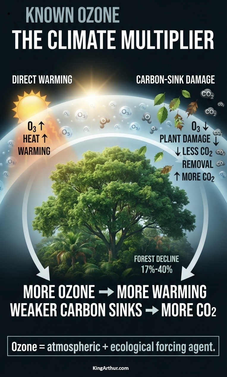
But ozone does something most greenhouse gases don’t: it also damages the plants that remove CO₂ from the atmosphere.

Ozone is a powerful phytotoxin—it harms plants. That creates an important climate feedback: the same ozone pollution that contributes directly to warming can damage vegetation, reduce photosynthesis, weaken carbon sequestration, and leave more CO₂ in the atmosphere.

Ozone is therefore both an atmospheric forcing agent and an ecological forcing agent.

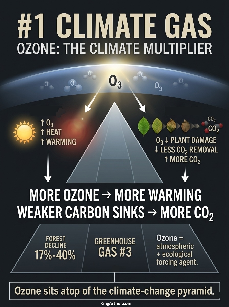
More ozone → more warming

and

More ozone → weaker carbon sinks → more CO₂ → more warming

That second pathway is the part of the ozone story that is often overlooked.


Ozone Damages Tropical Forests

A study published in Nature Geoscience, “Reduced productivity and carbon drawdown of tropical forests from ground-level ozone exposure,” found substantial reductions in tropical forest productivity associated with anthropogenic ground-level ozone exposure.

The study estimated that anthropogenic ozone pollution reduced tropical forest net primary productivity by approximately 17% globally since 2000.

That is a major climate consequence. Tropical forests are among Earth’s most important biological carbon sinks. When ozone reduces their productivity, their capacity to remove carbon from the atmosphere is reduced. Ozone has also been identified as one of the stressors contributing to the risk of Amazon forest dieback, alongside warming, drought, fire, and other interacting pressures.

The message is simple:

Ozone doesn’t just warm the planet. It can damage one of the planet’s major systems for removing CO₂.


Pennsylvania Forests Show the Warning Signs

Long-term observations of mature forests in Pennsylvania provide evidence of serious changes in forest health that warrant examination in the context of ozone exposure, climate stress, and carbon sequestration.

Since approximately 2003, observations across multiple monitoring intervals have reported substantial changes in some old-growth forest systems, including:

  • Approximately 40% foliage loss
  • Significant canopy thinning
  • Approximately 33% reductions in canopy height
  • Increased premature mortality

These changes cannot automatically be attributed to ozone alone. Forest decline is produced by interacting stresses, including ozone, heat, drought, hydrological disruption, insects, disease, and extreme weather. But that does not make ozone less important. It makes the interaction more important.

When multiple environmental stresses strike the same forest, ozone can become another force reducing the ability of vegetation to grow, survive, and store carbon.


The Ozone Multiplier

Ozone is therefore more than another greenhouse gas.

It can operate simultaneously through two pathways:

Atmospheric pathway

Ozone → greenhouse warming → more climate stress

Biological pathway

Ozone → plant damage → less photosynthesis → weaker carbon sinks → more atmospheric CO₂ → more warming

Put the two pathways together and ozone becomes a powerful climate multiplier.

The atmosphere warms the biosphere.

The biosphere normally removes CO₂ from the atmosphere.

Ozone interferes with that exchange.


Known Ozone

Ozone’s direct greenhouse effect is well established. Its ability to damage vegetation is also well established. The climate significance comes from putting those two facts together.

Ozone warms the planet.

Ozone damages plants.

Damaged plants remove less carbon.

Less carbon removal leaves more CO₂ in the atmosphere.

More CO₂ means more warming.

That makes ozone more than an air-pollution problem.

It makes ozone part of the climate feedback system itself.

And when the direct warming effect and the carbon-sink effect are considered together, ozone sits atop of the climate-change pyramid.

Known ozone.
Known warming.
Known plant damage.
Known powerful feedback.

Introduction to Ozone and Climate Change

Low-Level Ozone: The Invisible Climate Pollutant Threatening Human Health and Accelerating Global Warming

The Ozone Feedback Theory: Tropospheric Ozone as a Driver of Ecosystem Decline, Carbon Sink Failure, and Climate Acceleration

The Ozone Climate Feedback: Fossil Fuel Combustion, Methane Emissions, Wildfires, and Ecosystem Degradation as Drivers of Self-Reinforcing Global Warming

Lightning-Generated Tropospheric Ozone and Earth-System Feedbacks

Ozone as a Climate Multiplier: Key Coupling Agent in Chemistry–Climate Feedbacks

Ozone Feedbacks From Carbon Combustion: Tropospheric Ozone, Ecosystem Collapse, and the Failure of Biofuel Narratives 

Runaway Feedbacks and the Collapse of Natural Carbon Sinks: Emerging Evidence From Forests, Permafrost, and Tropospheric Ozone 

The Silent Unraveling of Forests: Ozone Stress, Climate Change, and Resilient Pennsylvania Tree Species

The Domino Collapse: Amazon Rainforest Dieback and the Ozone Feedback Loop

The Dangers of Tropospheric Ozone: A Silent Threat to Health and the Environment

SIMPLIFIED ANNOUNCEMENT

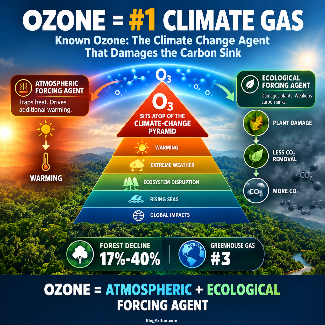
Ozone = #1 Climate Gas

Known Ozone: The Climate Change Agent That Damages the Carbon Sink

Ozone is usually treated as greenhouse gas #3.

But that misses the bigger picture.

Ozone sits atop the climate-change pyramid.

Why?

Because ozone is both an:

ATMOSPHERIC FORCING AGENT
→ traps heat
→ drives additional warming

and an:

ECOLOGICAL FORCING AGENT
→ damages plants
→ reduces photosynthesis
→ weakens carbon sinks
→ leaves more CO₂ in the atmosphere
→ drives additional warming

FOREST DECLINE: 17%–40%

GREENHOUSE GAS: #3

Ozone doesn’t just warm the atmosphere.

It can damage the biological systems that remove CO₂ from it.

OZONE = ATMOSPHERIC + ECOLOGICAL FORCING AGENT

That makes ozone one of the most important—and overlooked—climate-change agents.

Read Known Ozone: The Climate Change Agent That Damages the Carbon Sink.

bookmark_borderThe Methane Feedback

by Daniel Brouse

Methane feedback emissions are accelerating: methane emissions from climate feedbacks have shown an accelerated, record-breaking surge since around 2007, with a massive spike since 2020.

Global Methane & Climate Feedback Trends (2000–Present)

Era / YearsAvg. Atmospheric Growth RateClimate Feedback & Wetland StatusKey Scientific Discovery & Observations
The Stabilization Plateau
(2000–2006)
~0.5 ppb / year
(Near-zero or negative growth)
Stable Baselines:
Natural wetland and freshwater systems fluctuated within historic variations.
The Equilibrium Period: Atmospheric methane was thought to have permanently leveled off due to a balance between human emissions and atmospheric sink removal.
The Renewed Acceleration
(2007–2019)
~7.0 ppb / year
(Steady, significant rise)
Activation of Feedbacks:
Warming tropics and altered hydrology begin driving a steady increase in natural microbial activity.
The Inflection Point (2007): The plateau abruptly ended. Isotopic analysis of air samples revealed a distinct shift toward light carbon-13 signatures, proving natural microbial sources were playing a larger role than initially modeled.
The Extreme Feedback Spike
(2020–2022)
~15.2 ppb / year
(Record-shattering growth)
Feedback Explosion:
Heavy tropical rainfall patterns (prolonged La Niña) and intense boreal summers caused major wetland flooding and surges.
The Twin-Driver Crisis: Unprecedented spikes in 2020 (+14.8 ppb) and 2021 (+17.7 ppb). A temporary slowdown in the atmosphere’s chemical clean-up capacity (OH radicals) compounded with massive wetland emissions to create a perfect storm.
The Current Baseline
(2023–Present)
~7.1 ppb / year
(Moderated but highly elevated)
Hemispheric Shifts:
Severe droughts in South America temporarily suppressed tropical wetlands, but high-latitude boreal systems continue to expand.
Low-Latency Tracking: Global monitoring networks show that while growth returned to pre-2020 levels due to atmospheric sink recovery, total annual natural emissions are highly sensitive to climate shocks and remain locked in an active positive feedback loop.

The 2026 data highlights a critical new development in atmospheric methane monitoring: while the extreme record-shattering growth rates seen in 2020–2021 have stabilized, total global methane concentrations have reached an all-time high, heavily sustained by strong natural feedback loops.

Ultimately, the data shows that human mitigation efforts are currently in a dead heat against escalating climate-driven natural feedbacks.

bookmark_borderClean Energy Economy

by Daniel Brouse

THE ENERGY IS ALREADY THERE.
THE CLEAN ENERGY ECONOMY HARVESTS IT.

Tonight’s homework assignment: Clean Energy Economy.

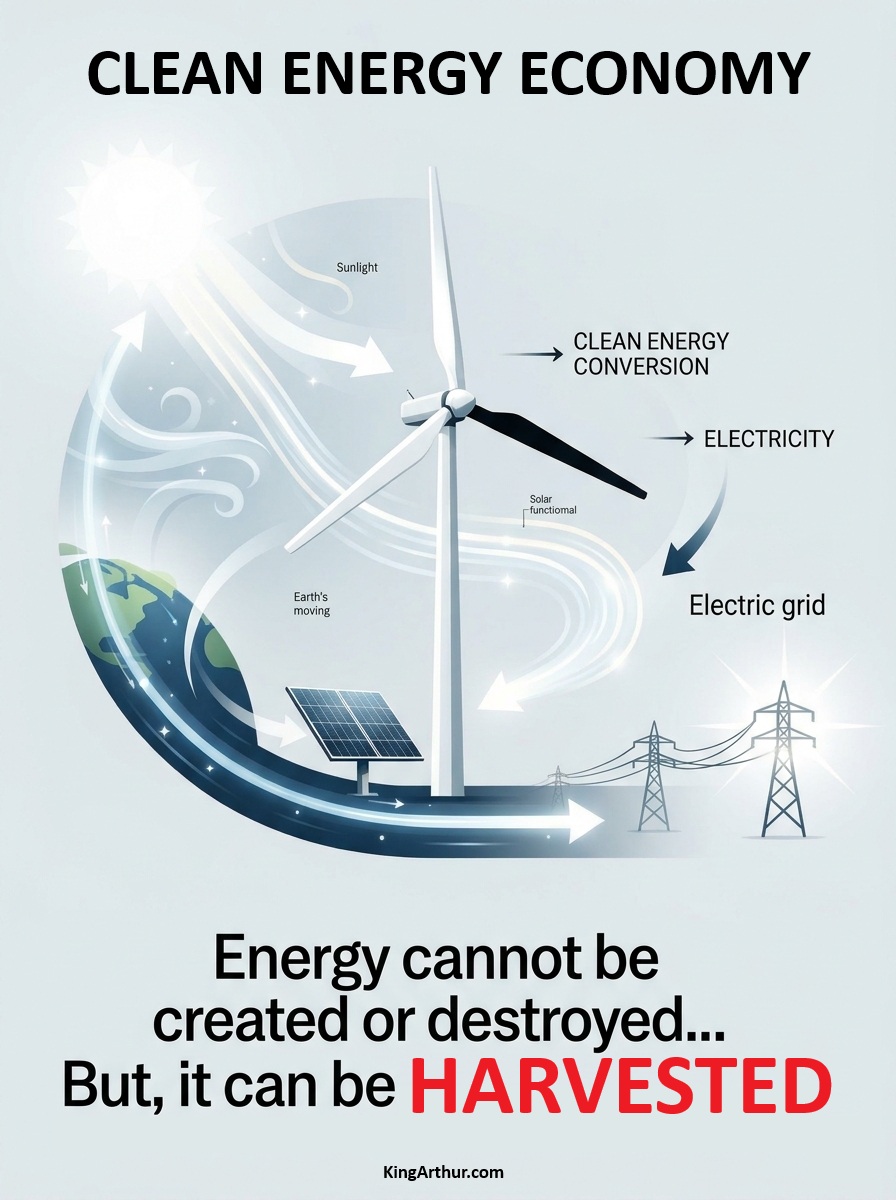
Energy cannot be created or destroyed. But it can be harnessed, converted, stored, transmitted, and used.

The sun is already delivering enormous amounts of energy to Earth.

The atmosphere is already moving.

Winds are already blowing.

Waves and currents are already moving.

The challenge isn’t creating energy from nothing. It is building systems that efficiently capture naturally available energy and convert it into useful electricity.

That is the basic idea behind a clean energy economy:

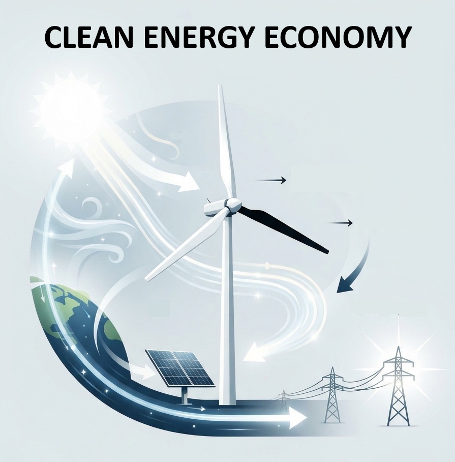
SUN + WIND + MOVING EARTH
↓
ENERGY HARVESTING
↓
ELECTRICITY
↓
STORAGE + TRANSMISSION
↓
USEFUL WORK

A wind turbine doesn’t create wind. A solar panel doesn’t create sunlight.

They harvest energy that is already moving through the Earth system and convert it into a form we can use.

The economic opportunity is therefore not simply replacing one fuel with another.

It is building an economy around capturing, converting, distributing, storing, and using energy that is already available.

THE ENERGY IS ALREADY THERE.

THE CLEAN ENERGY ECONOMY HARVESTS IT.

bookmark_borderChange in Climate Change: Δc

by Daniel Brouse and Sidd Mukherjee

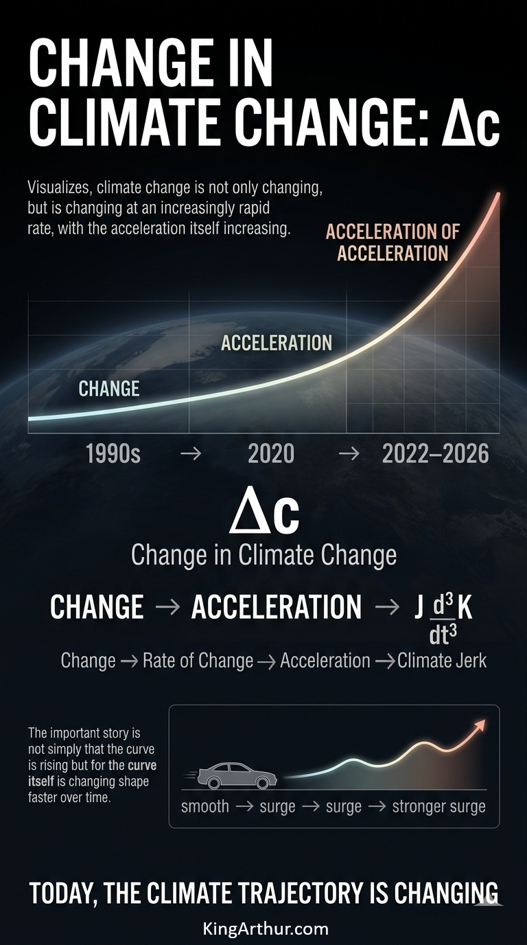
Since the ’90s, we’ve been in pursuit of change in climate change (Δc).

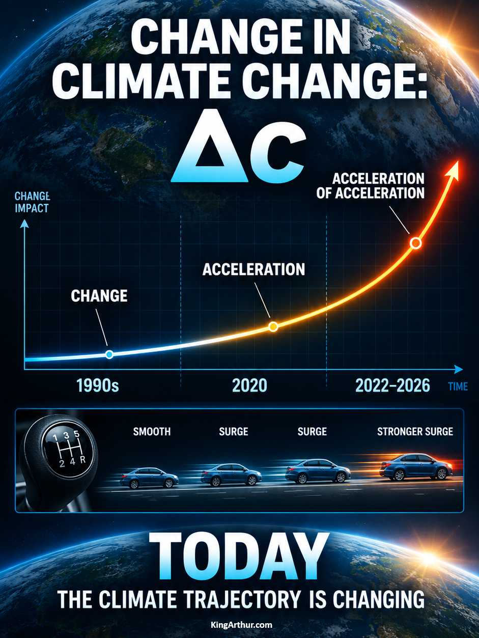
It took us about 10 years to recognize that the rate of change was doubling on roughly a 100-year timescale.

By 2020, the acceleration in acceleration had changed substantially: the doubling interval had compressed to roughly 10–20 years.

That represents a 5–10× increase in the rate of doubling—or, expressed on a centurial basis, a shift from 2¹ to roughly 2⁵–2¹⁰.

Beginning most notably around 2022, we began seeing something different happening in the climate system. Several major climate variables started changing together, in ways that were physically connected. It was no longer just a matter of the climate getting warmer—it was the parts of the climate system increasingly interacting with and reinforcing one another in real time.

At the same time, an extraordinary number of extreme climate events were being documented and rapidly shared through social-media platforms, providing additional real-world observations of climate-system behavior. Among the most striking examples was the Nepal–Tibet glacial collapse.

The models consistently produced similar results.

The period from 2022–2026 exhibits what mathematicians describe as third-derivative, or “jerk,” behavior: the rate of acceleration is itself changing at an accelerating rate, producing a nonlinear trajectory.

A simple analogy is sitting in the passenger seat while someone learns to drive a stick shift. Instead of a smooth increase in speed, you feel the repeated surges and lurches as the driver learns to coordinate the clutch, throttle, and gears. The acceleration is changing—and the rate at which that acceleration changes is changing as well.

That is the essential idea behind climate jerk: not simply that the climate system is changing faster, but that the acceleration of change is itself accelerating.