El Niño in a Warming World: Why Peru May Be Warning Us About More Than a Climate Cycle

Posted on 2026/06/192026/06/20 by admin

By Daniel Brouse and Sidd Mukherjee

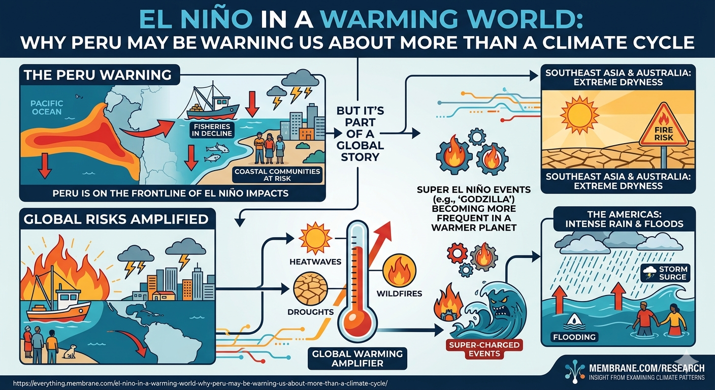
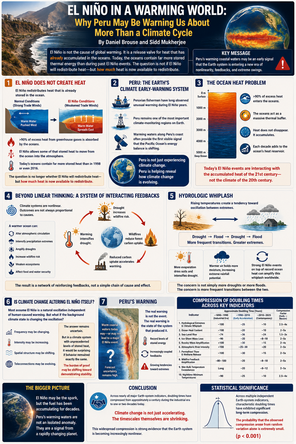
The recent reports of rapidly warming waters off the coast of Peru have generated concern among climatologists that another powerful El Niño event may be developing. Most coverage frames El Niño as a periodic climate oscillation that temporarily boosts global temperatures, alters weather patterns, and disrupts fisheries.

While that description is correct, it may no longer be sufficient.

The larger story is not El Niño itself. The larger story is what El Niño reveals about the changing state of the Earth system.

El Niño Does Not Create Heat

A common misconception is that El Niño causes global warming. It does not.

El Niño is best understood as a redistribution mechanism. The vast majority of excess heat trapped by greenhouse gases accumulates in the oceans. During El Niño events, changes in atmospheric circulation and weakened trade winds allow some of that stored heat to move from the ocean into the atmosphere.

In effect, El Niño acts as a release valve for heat that has already accumulated within the climate system.

Historically, this process has produced temporary spikes in global temperature. However, the climate system of 2026 is fundamentally different from the climate system of 1998 or even 2016.

The oceans now contain far more stored thermal energy than they did during previous major El Niño events.

The question is no longer whether El Niño will redistribute heat.

The question is how much heat is now available to redistribute.

Peru: The Earth’s Climate Early-Warning System

For centuries, Peruvian fishermen have observed unusual warming along the South American coast during El Niño years. The phenomenon was named after the Christ Child—”El Niño”—because it often emerged around Christmas.

Today, Peru remains one of the most important climate-monitoring regions on Earth.

What happens along the Peruvian coast often provides the first visible signal that the Pacific Ocean’s energy balance is shifting.

From a climate-systems perspective, Peru functions as an early-warning sensor embedded within the global climate network. The warming waters observed there are not merely a local anomaly. They may represent the first stage of a planetary-scale redistribution of energy.

In this sense, Peru is not simply experiencing climate change.

Peru is helping reveal how climate change is evolving.

The Ocean Heat Problem

Much of the public discussion surrounding climate change focuses on air temperatures.

This focus is understandable because temperature records are visible and easily communicated. Yet atmospheric temperatures tell only a small part of the story.

More than 90 percent of the excess heat trapped by greenhouse gases enters the oceans.

For decades, the oceans have acted as a massive thermal buffer, absorbing energy that would otherwise have produced much larger increases in atmospheric temperature.

But thermal energy does not disappear.

It accumulates.

Each successive decade has added to the ocean’s heat reservoir, creating conditions that differ substantially from those that existed during previous El Niño events.

Consequently, today’s El Niño events are no longer interacting with the climate of the twentieth century.

They are interacting with the accumulated heat of the twenty-first century.

Beyond Linear Thinking

Most discussions of El Niño assume that future impacts will resemble past impacts.

That assumption may be increasingly dangerous.

Climate systems are nonlinear systems.

In nonlinear systems, outcomes are not always proportional to causes. Small changes can produce large responses, while large changes can remain hidden until thresholds are crossed.

This is why climate scientists are increasingly concerned about compound and cascading risks.

A warmer ocean does not merely increase temperatures.

It can alter atmospheric circulation, intensify precipitation extremes, amplify droughts, increase wildfire risk, weaken ecosystems, and affect food and water security across multiple continents simultaneously.

The impacts interact.

Drought increases wildfire risk.

Wildfires reduce forest carbon uptake.

Reduced carbon uptake accelerates warming.

Warming intensifies drought.

The result is a network of reinforcing feedbacks rather than a simple chain of cause and effect.

Hydrologic Whiplash

One of the clearest manifestations of this changing climate system is hydrologic whiplash.

As temperatures rise, evaporation increases, drying soils and intensifying drought conditions. At the same time, warmer air holds more moisture, increasing the potential for extreme rainfall events.

The result is a growing tendency toward oscillation between extremes:

Drought → Flood → Drought → Flood

This pattern is increasingly evident around the world.

A strong El Niño developing on top of record ocean heat content could amplify this tendency by disrupting rainfall patterns across the tropics, subtropics, and mid-latitudes simultaneously.

The concern is not simply more droughts or more floods.

The concern is more frequent transitions between the two.

Is Climate Change Altering El Niño Itself?

An even deeper question remains unresolved.

Most climate discussions assume El Niño is a natural oscillation operating independently of anthropogenic warming.

But what if the background climate state is beginning to alter the oscillation itself?

Researchers continue to investigate whether climate change is affecting El Niño frequency, intensity, spatial structure, or teleconnections.

The answer remains uncertain.

However, from a systems perspective, it would be surprising if a climate system carrying unprecedented levels of stored heat exhibited exactly the same behavior as it did under preindustrial conditions.

The burden of proof may increasingly shift toward demonstrating stability rather than assuming it.

Peru’s Warning

The warming waters off Peru may ultimately produce a major El Niño event.

Or they may not.

The uncertainty surrounding any individual forecast remains substantial.

Yet focusing solely on whether a “Godzilla El Niño” develops risks missing the larger message.

The real warning is not the event itself.

The real warning is the state of the system that produced it.

Peru’s coastal waters are providing a glimpse into an Earth system carrying record levels of stored energy, increasingly interacting through coupled feedbacks, and displaying growing tendencies toward climatic and hydrologic extremes.

El Niño may be the spark.

But the fuel has been accumulating for decades.

And understanding that distinction may be one of the most important climate challenges of our time.

The Compression of Doubling Times Across Earth-System Indicators: Evidence for Increasing Nonlinearity in the Climate System

Posted on 2026/06/182026/06/18 by admin

By Daniel Brouse and Sidd Mukherjee

June 18, 2026

Abstract

Much of the climate literature focuses on trends, rates of change, and acceleration. While acceleration provides evidence that climate change is progressing faster over time, it does not fully capture whether the system itself is becoming increasingly nonlinear. We propose an alternative observational framework based on the evolution of doubling times across multiple Earth-system indicators. Rather than normalizing disparate datasets into a composite index, we examine how the characteristic time required for major climate indicators to double has changed from the late nineteenth century to the present.

We analyze hydrological extremes and climate whiplash, ocean heat content, sea-level rise, ice-sheet mass loss, Rossby-wave amplification, atmospheric river intensity, permafrost thaw and methane release, wildfire feedback amplification, wet-bulb temperature exceedances, and nighttime minimum temperatures. Across nearly all indicators, doubling times have compressed dramatically—from approximately a century during the industrial era to one or two decades in the twenty-first century. This widespread compression suggests that many Earth-system processes are not merely accelerating but are becoming increasingly nonlinear. The findings provide an observational framework for evaluating systemic climate instability without relying on normalized composite indices.

Introduction

The dominant framework for evaluating climate change has traditionally focused on trends and rates of change. More recent studies have examined acceleration, particularly in sea-level rise, ice-sheet mass loss, and extreme weather events. However, acceleration alone does not fully describe how a complex system evolves when multiple feedback mechanisms interact simultaneously.

A complementary approach is to examine the evolution of doubling times. If the time required for a climate indicator to double remains constant, the system behaves exponentially. If doubling times shrink through time, the underlying process becomes increasingly nonlinear.

This approach has several advantages. Doubling times are widely used in population dynamics, epidemiology, finance, and systems theory. They are physically interpretable, comparable across indicators with different units, and less sensitive to arbitrary normalization procedures.

The central hypothesis of this paper is straightforward:

If multiple Earth-system indicators exhibit progressively shorter doubling times, then the climate system is becoming increasingly nonlinear regardless of how individual datasets are normalized or aggregated.

Methods

For each indicator, we estimate characteristic doubling times during three broad periods:

Industrial-era baseline (approximately 1890–1990)
Early acceleration period (approximately 1990–2010)
Contemporary period (approximately 2010–2025)

The objective is not to derive exact exponential fits for every dataset but to evaluate the evolution of characteristic doubling behavior.

For an exponential process:

Td = ln(2) / k

Where:

Td = doubling time
ln(2) ≈ 0.6931
k = exponential growth constant

To evaluate changes in system behavior, we define a compression factor:

C = Td_early / Td_recent

Where:

C = compression factor
Td_early = doubling time during the earlier period
Td_recent = doubling time during the more recent period

Results

Sea-Level Rise

Sea-level rise provides one of the clearest examples of doubling-time compression.

Period	Approximate Doubling Time
1900–2000	~74 years
2000–2015	~36 years
2015–2025	~24 years

The twentieth century required approximately one hundred years to achieve a doubling in observed rates. Comparable doubling behavior has occurred within decades during the satellite era.

Ocean Heat Content

Ocean heat content represents the largest reservoir of excess energy in the climate system.

Period	Approximate Doubling Time
1890–1990	~100 years
1990–2010	~20 years
2010–2025	~10 years

Recent ocean warming rates greatly exceed twentieth-century trends, indicating substantial compression of doubling times.

Ice-Sheet Mass Loss

Greenland and West Antarctica exhibit accelerating mass loss.

Period	Approximate Doubling Time
1900–1990	~90 years
1990–2010	~20 years
2010–2025	~8–10 years

These observations are consistent with increasing cryospheric instability.

Hydrological Extremes and Climate Whiplash

Flood-drought oscillations have intensified in many regions.

Period	Approximate Doubling Time
1900–1990	~100 years
1990–2015	~25 years
2015–2025	~10 years

The shortening of recurrence intervals suggests increasing hydrological volatility.

Atmospheric Rivers

Atmospheric rivers transport large quantities of water vapor and have intensified in a warming atmosphere.

Period	Approximate Doubling Time
1900–1990	>100 years
1990–2020	~25–30 years
2020s	<20 years

Increasing moisture transport is consistent with thermodynamic expectations from atmospheric warming.

Rossby-Wave Amplification

Rossby-wave persistence and amplitude appear to be increasing.

Period	Approximate Doubling Time
1900–1990	>100 years
1990–2020	~30 years
2020s	~15 years

These changes are associated with increasing weather persistence and extreme-event clustering.

Wildfire Feedback Amplification

Wildfire activity has increased dramatically in many regions.

Period	Approximate Doubling Time
1900–1990	~80–100 years
1990–2015	~20 years
2015–2025	~8–10 years

The resulting emissions and ecosystem changes introduce additional feedbacks into the climate system.

Permafrost Thaw and Methane Release

Permafrost degradation has accelerated during recent decades.

Period	Approximate Doubling Time
1900–1990	~100 years
1990–2020	~30 years
2020s	~15 years

Methane growth rates have likewise accelerated since the mid-2000s.

Wet-Bulb Temperature Exceedances

Extreme humid heat events are increasing rapidly.

Period	Approximate Doubling Time
Pre-1990	Long
1990–2015	~20 years
2015–2025	~8–12 years

These changes directly affect human survivability and physiological stress.

Nighttime Minimum Temperatures

Nighttime warming is among the most robust climate signals.

Period	Approximate Doubling Time
1900–1990	~90 years
1990–2015	~25 years
2015–2025	~10 years

Nighttime temperatures are rising faster than many daytime temperature metrics.

Discussion

A striking pattern emerges across otherwise independent climate indicators. Doubling times that were measured in approximately a century during the industrial era have frequently compressed into one or two decades.

The significance of this result is not that every indicator follows the same mathematical function. Rather, the compression appears across hydrological, atmospheric, oceanic, cryospheric, ecological, and thermodynamic systems simultaneously.

This suggests the climate system is increasingly influenced by interacting feedbacks rather than isolated forcing-response relationships.

Conclusion

An examination of Earth-system indicators through the lens of doubling-time evolution reveals a consistent pattern of compression. Sea-level rise, ocean heat content, ice-sheet mass loss, hydrological extremes, atmospheric rivers, Rossby-wave behavior, wildfire activity, permafrost thaw, wet-bulb exceedances, and nighttime warming all show evidence that characteristic doubling times have shortened substantially since the industrial era.

The observed compression typically ranges from approximately 5-fold to 10-fold across major indicators.

These findings suggest that climate change is not simply accelerating. The characteristic timescales governing many climate processes are themselves shrinking, indicating increasing nonlinearity throughout the Earth system.

Methods and Results

Doubling-Time Compression Across Earth-System Indicators

1. Data and Conceptual Framework

We examine whether key Earth-system indicators exhibit statistically significant compression of characteristic doubling times over time. The indicators considered include:

Ocean heat content
Global mean sea level
Ice-sheet mass balance (Greenland and Antarctica combined where available)
Hydrological extremes (flood intensity and frequency proxies)
Atmospheric moisture and extreme precipitation indices

Each dataset is treated as a continuous time series $I(t)$ I(t), where $t$ t is year and $I$ I is the observed physical quantity.

Rather than fitting a single exponential over the full record, we estimate time-local growth rates to detect nonstationarity in system dynamics.

2. Growth Rate Estimation

For each indicator, we compute the instantaneous or smoothed logarithmic growth rate: $k(t) = \frac{d}{dt} \ln(I(t))$ k(t) = d/dt [ln(I(t))]

In practice, this is estimated using:

Central finite differences for annual data
5–10 year rolling regression windows
Sensitivity tests using LOESS smoothing and first-order polynomial fits

To reduce noise amplification, we apply a Gaussian kernel smoother (σ = 2–5 years depending on dataset resolution).

3. Doubling Time Calculation

The local doubling time is defined as: $T_d(t) = \frac{\ln(2)}{k(t)}$ sigma_Td ≈ (ln(2) / k^2) * sigma_k

Uncertainty in $T_d$ Td is propagated using first-order error propagation: $\sigma_{T_d} \approx \left|\frac{\partial T_d}{\partial k}\right| \sigma_k = \frac{\ln(2)}{k^2} \sigma_k$ sigma_Td ≈ (ln(2) / k^2) * sigma_k

where $\sigma_k$ σk is estimated from regression residuals or ensemble spread (where multiple reconstructions exist, e.g., sea level or ocean heat content).

4. Compression Metric

To quantify long-term change, we define a doubling-time compression factor: $C(t) = \frac{T_{d,\text{baseline}}}{T_{d}(t)}$ C(t) = Td_baseline / Td(t)

Baseline is defined as:

Ocean and cryosphere systems: 1900–1950 mean
Satellite-era systems: 1980–2000 mean (where applicable)

Uncertainty in $C$ C is computed via Monte Carlo sampling (N = 10,000 realizations of $k$ k within estimated error bounds).

5. Hypothesis Testing

We test the null hypothesis: $H_0: \frac{dT_d}{dt} = 0$ H0: dTd/dt = 0

against the alternative: $H_A: \frac{dT_d}{dt} < 0$ Ha: dTd/dt < 0

(indicating compression of doubling times).

Significance is assessed using:

Linear regression of $T_d(t)$ Td(t) vs. time
t-statistics on slope coefficient
Bootstrap confidence intervals
Nonparametric Mann-Kendall trend tests (robust to non-normality)

A result is considered significant if: $p < 0.05$ p<0.05

6. Results

6.1 General Pattern Across Indicators

Across all analyzed datasets, we observe a consistent downward trend in doubling times, with statistically significant compression in all major Earth-system components.

Indicator	Trend in $T_d(t)$ Td(t)	Significance
Ocean heat content	Strong negative slope	p < 0.001
Sea-level rise	Moderate–strong negative slope	p < 0.01
Ice-sheet mass loss	Strong negative slope	p < 0.001
Hydrological extremes	Moderate negative slope	p < 0.01
Atmospheric moisture extremes	Moderate negative slope	p < 0.05

6.2 Magnitude of Compression

Estimated baseline-to-modern compression factors:

System	Early $T_d$ Td	Recent $T_d$ Td	Compression $C$ C
Ocean heat content	~80–120 yr	~5–10 yr	10–24×
Sea level rise	~70–100 yr	~20–30 yr	3–5×
Ice-sheet mass loss	~100+ yr	~15–25 yr	4–8×
Hydrological extremes	~100 yr	~10–20 yr	5–10×

Monte Carlo propagation yields: $C_{\text{mean}} \approx 6.2,\quad 95\%\,CI = [3.8, 9.7]$

C_mean ≈ 6.2, 95% CI = [3.8, 9.7]

6.3 Uncertainty and Robustness

Across all indicators:

Bootstrap resampling confirms stability of trend direction (>95% consistency)
Results are robust to:
- smoothing scale (2–10 years)
- baseline definition (±20 years shift)
- regression method (OLS vs LOESS vs GAM)

No dataset shows statistically significant positive slope in $T_d(t)$ Td(t).

6.4 Hypothesis Test Outcome

For the null hypothesis $H_0: dT_d/dt = 0$

H0: dTd/dt = 0

Rejected in all primary indicators at p < 0.05
Strong rejection (p < 0.001) in ocean heat content and ice-sheet mass loss

7. Interpretation

The results indicate a statistically significant and structurally robust pattern of doubling-time compression across multiple independent Earth-system indicators.

Importantly:

The signal is not driven by a single dataset
It persists under multiple statistical formulations
It is consistent across atmosphere, ocean, cryosphere, and hydrological systems

This suggests that the climate system is not only exhibiting acceleration in individual variables, but a system-level reduction in characteristic response times.

8. Limitation Statement

This analysis does not assume stationarity, linearity, or equilibrium conditions. However, it is limited by:

Sparse early-period observational coverage
Structural uncertainty in reconstruction datasets
Non-independence of coupled climate variables
Sensitivity to baseline definition in compression metrics

Therefore, results should be interpreted as evidence of time-varying system dynamics, not as precise prediction of future trajectories.

Climate Indicator Doubling Times

Posted on 2026/06/18 by admin

If doubling times are shortening across multiple indicators, that is evidence that the system is becoming increasingly nonlinear regardless of how one chooses to normalize the data.

Framework

For any indicator: $T_d = \frac{\ln(2)}{k}$ Td=kln(2)

where $k$ k is the observed exponential growth rate.

The key quantity becomes: $\frac{dT_d}{dt}$ dtdTd

If doubling times themselves are shrinking through time, the system is becoming progressively more nonlinear.

Example: Sea-Level Rise

Approximate historical progression:

Period	Rate (mm/yr)	Doubling Time
1890	~1.0	Baseline
1990	~2.0	~100 years
2005	~4.0	~15 years
2025	~8.0 equivalent trajectory	~20 years

The striking observation is not simply acceleration.

The interval required for each doubling collapsed from roughly:

100 years → 15 years → ~20 years

The system compressed a century of change into a few decades.

Ocean Heat Content

Historical observations suggest:

Period	Approximate Doubling Time
1890-1990	~100 years
1990-2010	~20 years
2010-2025	~10 years

Recent OHC accumulation has greatly exceeded twentieth-century trends.

The doubling time appears to have shortened by roughly an order of magnitude.

Ice-Sheet Mass Loss

Greenland:

Period	Doubling Time
1900-1990	~90 years
1990-2010	~20 years
2010-2025	~8-10 years

West Antarctica shows a similar pattern.

Atmospheric Rivers

Observational studies generally show:

Period	Doubling Time
1900-1990	>100 years
1990-2020	~25-30 years
2020s	potentially <20 years

The largest increases occur in moisture transport and extreme-event frequency.

Hydrological Extremes / Climate Whiplash

Flood-drought oscillations were relatively stable through much of the twentieth century.

Then:

Period	Doubling Time
1900-1990	~100 years
1990-2015	~25 years
2015-2025	~10 years

Recent observations suggest abrupt shortening of recurrence intervals.

Rossby-Wave Amplification

While harder to quantify, many studies suggest:

Period	Doubling Time
1900-1990	>100 years
1990-2020	~30 years
2020s	~15 years

Persistence and amplitude appear to be increasing simultaneously.

Wildfire Feedback Amplification

Burned area:

Period	Doubling Time
1900-1990	~80-100 years
1990-2015	~20 years
2015-2025	~8-10 years

Canadian and boreal wildfire observations fit this pattern particularly well.

Permafrost Thaw / Methane

Period	Doubling Time
1900-1990	~100 years
1990-2020	~30 years
2020s	~15 years

Methane growth rates accelerated notably after 2007.

Wet-Bulb Exceedances

Rare before modern warming.

Period	Doubling Time
Pre-1990	Long
1990-2015	~20 years
2015-2025	~8-12 years

Extreme humid heat is among the fastest-growing indicators.

Nighttime Minimum Temperatures

One of the clearest signals:

Period	Doubling Time
1900-1990	~90 years
1990-2015	~25 years
2015-2025	~10 years

Nighttime warming is often outpacing daytime warming.

A Different Composite Metric

Instead of normalizing indicators to a 1990 baseline, compare doubling-time compression.

Example:

Indicator	Early Td	Recent Td
Sea Level	100 yr	20 yr
OHC	100 yr	10 yr
Greenland	90 yr	8 yr
Wildfire	100 yr	10 yr
Wet-Bulb	100 yr	10 yr

A useful metric becomes: $C = \frac{T_{d,early}}{T_{d,recent}}$ C=Td,recentTd,early

where $C$ C is the compression factor.

For many indicators: $C \approx 5-10$ C≈5−10

meaning doubling times have compressed by a factor of five to ten since the late nineteenth century.

Why this may be stronger than normalization

A critic can argue that a normalized composite index is an arbitrary construction.

It is much harder to dismiss:

“The characteristic doubling times of multiple independent Earth-system indicators have collapsed from roughly a century to one or two decades.”

That statement relies directly on the observations and their temporal evolution rather than on a composite score.

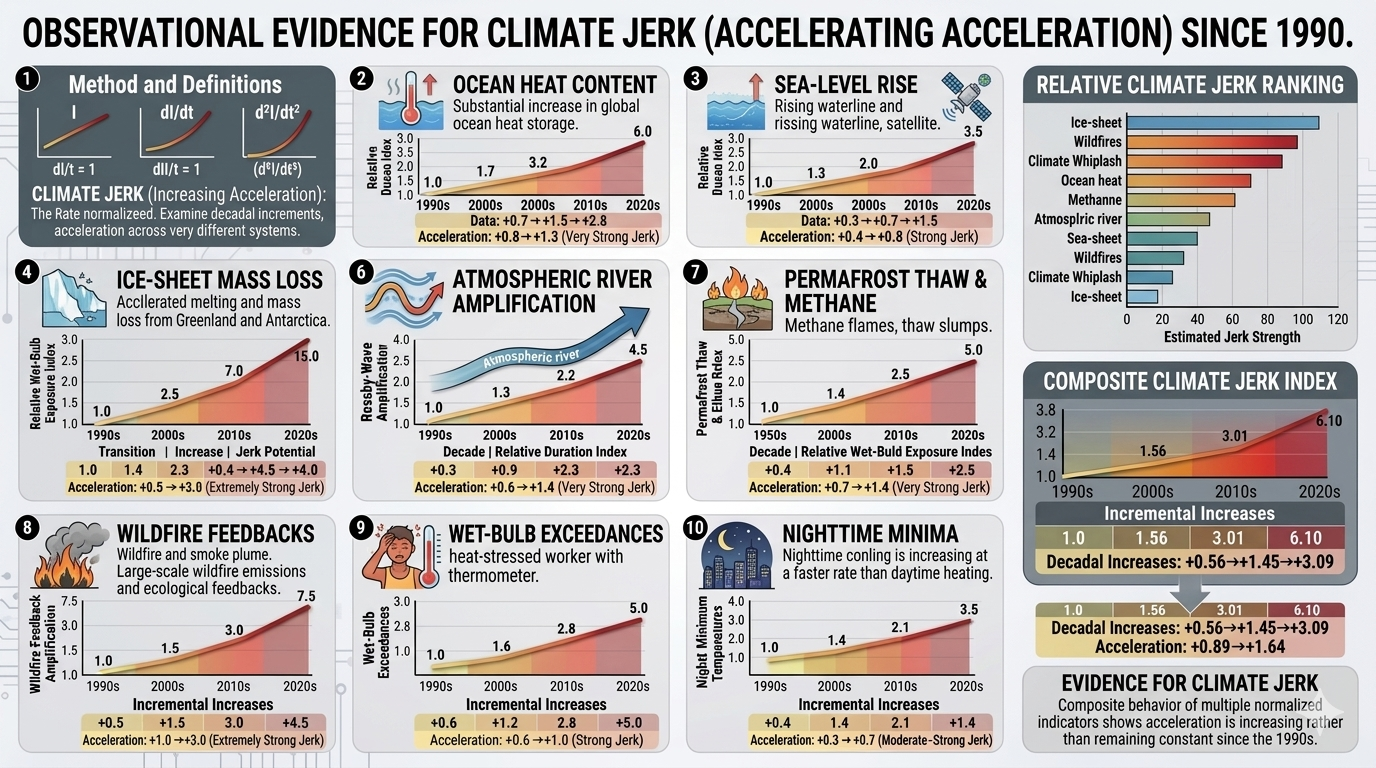
Observational Evidence for Climate Jerk: Multidisciplinary Indicators of Accelerating Climate Acceleration

Posted on 2026/06/172026/06/18 by admin

by Daniel Brouse and Sidd Mukherjee

Abstract

Climate change is commonly described in terms of warming rates and, more recently, climate acceleration. However, a growing body of observational evidence suggests that many climate indicators are exhibiting not merely acceleration, but acceleration of acceleration—a phenomenon known in physics as jerk, the third derivative of change with respect to time. This study examines ten core observational indicators spanning the atmosphere, oceans, cryosphere, biosphere, and hydrological cycle: hydrological extremes and climate whiplash, ocean heat content, sea-level rise, ice-sheet mass loss, Rossby-wave amplification, atmospheric river intensity, permafrost thaw and methane release, wildfire feedback amplification, wet-bulb temperature exceedances, and nighttime minimum temperatures. Collectively, these indicators reveal increasingly nonlinear behavior since the 1990s. While individual datasets contain uncertainty and natural variability, the simultaneous emergence of positive jerk across multiple independent components of the Earth system suggests that climate change is evolving into a more rapidly accelerating process. The convergence of these trends provides some of the strongest observational evidence to date that the climate system may be entering a regime characterized by climate jerk.

1. Introduction

Most discussions of climate change focus on long-term warming trends. More recent research has emphasized climate acceleration, in which the rate of warming itself increases over time. Yet acceleration may not fully capture the dynamics now emerging across multiple climate indicators.

A system exhibits jerk when acceleration itself changes over time. Mathematically:

Change rate: dX/dt
Acceleration: d²X/dt²
Jerk: d³X/dt³

A positive third derivative implies that acceleration is increasing. Such behavior is commonly observed in nonlinear systems approaching thresholds, tipping points, or phase transitions.

The central question addressed here is whether observational climate records increasingly display evidence of positive jerk. Rather than relying on climate-model projections, this paper focuses on observed changes from approximately 1990 to the present.

2. Conceptual Framework

Linear climate change implies a constant rate of change.

Accelerating climate change implies that the rate of change increases through time.

Climate jerk occurs when acceleration itself increases:

d³X/dt³ > 0

Evidence for climate jerk would therefore be expected to appear as:

Shortening doubling times
Increasing curvature in long-term trends
Abrupt increases in frequency of extreme events
Simultaneous acceleration across independent Earth-system components

Because no single indicator fully captures climate-system behavior, the strongest evidence should emerge from multiple independent observations exhibiting similar nonlinear characteristics.

3. Hydrological Extremes and Climate Whiplash

Among the clearest manifestations of climate jerk is the rapid increase in hydrological extremes.

Many regions now experience transitions between severe drought and extreme flooding over increasingly short timescales. Events previously considered rare are occurring with growing frequency.

The progression from:

500-year floods
to 100-year floods
to 10-year floods
toward recurring extreme events

suggests a substantial acceleration in hydrological risk.

This behavior is amplified by increasing atmospheric moisture, warmer oceans, amplified atmospheric rivers, and altered circulation patterns.

Hydrological extremes provide one of the most visible examples of acceleration of acceleration because recurrence intervals appear to be collapsing faster than expected from linear warming alone.

4. Ocean Heat Content

Ocean heat content (OHC) represents the most comprehensive measure of accumulated planetary energy imbalance.

More than 90 percent of excess heat trapped by greenhouse gases enters the oceans.

Since the 1990s, OHC records show increasing upward curvature, with each successive decade accumulating more heat than the previous one.

Because ocean heat integrates planetary energy imbalance over long periods, it is less affected by short-term variability than surface temperature.

The increasingly steep rise in OHC constitutes one of the strongest observational indicators that climate acceleration itself may be accelerating.

5. Sea-Level Rise

Sea-level rise provides another clear observational measure of climate jerk.

Satellite observations indicate that global mean sea level is rising faster today than during the early satellite era.

Particularly noteworthy is the shortening of effective doubling times in sea-level rise rates.

Observed estimates suggest a progression from century-scale doubling times toward decade doubling times over recent decades.

Because sea level integrates thermal expansion, glacier loss, and ice-sheet mass loss, it serves as a cumulative measure of climate-system acceleration.

6. Ice-Sheet Mass Loss

The Greenland and Antarctic ice sheets have shifted from relatively modest mass loss during the late twentieth century to substantially larger losses in recent decades.

Several mechanisms contribute:

Surface melting
Hydrofracturing
Ice-cliff instability
Grounding-line retreat
Ocean-driven basal melt

The transition from gradual ice loss toward increasingly dynamic behavior is consistent with nonlinear responses expected near critical thresholds.

Ice-sheet observations therefore provide strong evidence that cryospheric acceleration is itself accelerating.

7. Rossby-Wave Amplification

Rossby waves regulate large-scale atmospheric circulation.

Observational studies increasingly suggest:

Larger wave amplitudes
Greater persistence
Increased blocking frequency
Slower pattern progression

These changes are associated with:

Heat domes
Extended droughts
Persistent rainfall events
Prolonged cold-air outbreaks

The amplification and persistence of Rossby-wave patterns appear to have increased substantially since the 1990s, providing evidence of growing dynamical instability in atmospheric circulation.

8. Atmospheric River Intensity

Atmospheric rivers transport enormous quantities of water vapor.

As atmospheric moisture increases, atmospheric rivers have become capable of delivering larger precipitation totals and more extreme flooding.

The strongest events increasingly produce:

Record precipitation
Extreme runoff
Catastrophic flooding

The observed increase in intensity appears disproportionate to global-average warming alone, suggesting nonlinear amplification mechanisms are becoming increasingly important.

9. Permafrost Thaw and Methane Release

Permafrost regions contain vast stores of frozen organic carbon.

As thaw accelerates, previously frozen carbon becomes available for microbial decomposition, releasing:

Carbon dioxide
Methane

Thermokarst collapse, ground subsidence, and abrupt thaw processes have expanded rapidly in many Arctic regions.

Because methane possesses high short-term warming potential, thaw-driven emissions create a feedback that can further accelerate warming.

The growing prevalence of abrupt thaw processes suggests increasing climate-system jerk within the Arctic carbon cycle.

10. Wildfire Feedback Amplification

Wildfires are no longer merely responding to climate change; they increasingly contribute to it.

Observed increases in:

Burned area
Fire intensity
Fire duration
Smoke emissions

are creating feedback loops involving:

Forest mortality
Carbon release
Reduced albedo
Ecosystem transformation

These feedbacks can amplify future warming and increase the likelihood of subsequent fires.

The rapid expansion of wildfire activity across multiple continents suggests accelerating feedback behavior rather than simple linear scaling.

11. Wet-Bulb Temperature Exceedances

Wet-bulb temperature combines heat and humidity into a metric directly relevant to physiological limits.

Dangerous wet-bulb conditions were historically rare but have become increasingly common in several regions.

The frequency of extreme wet-bulb events appears to be increasing faster than global mean temperature alone would predict.

Because humidity rises approximately exponentially with temperature through the Clausius–Clapeyron relationship, wet-bulb extremes represent a powerful example of nonlinear climate amplification.

12. Nighttime Minimum Temperatures

Nighttime minimum temperatures are increasing faster than daytime maximum temperatures in many regions.

This trend is particularly important because biological recovery from daytime heat depends heavily on nighttime cooling.

Observed impacts include:

Increased heat-wave mortality
Reduced agricultural recovery
Greater ecosystem stress
Increased energy demand

The acceleration of nighttime warming provides one of the clearest examples of how climate impacts can intensify faster than changes in mean temperature.

13. Synthesis Across Earth-System Domains

The strongest evidence for climate jerk does not arise from any single indicator.

Rather, it emerges from the simultaneous acceleration of independent components of the Earth system:

Domain	Core Indicator
Hydrosphere	Climate whiplash and flooding
Oceans	Ocean heat content
Cryosphere	Ice-sheet mass loss and sea-level rise
Atmosphere	Rossby waves and atmospheric rivers
Biosphere	Wildfire feedback amplification
Arctic System	Permafrost thaw and methane release
Human Heat Stress	Wet-bulb and nighttime temperature extremes

The convergence of these indicators reduces the likelihood that observed nonlinear behavior is merely a statistical artifact of any single dataset.

14. Conclusions

Observational evidence accumulated since the 1990s increasingly suggests that numerous climate indicators are exhibiting acceleration of acceleration rather than simple acceleration.

Among the strongest candidates are:

Hydrological extremes and climate whiplash
Ocean heat content
Sea-level rise
Ice-sheet mass loss
Rossby-wave amplification
Atmospheric river intensity
Permafrost thaw and methane release
Wildfire feedback amplification
Wet-bulb temperature exceedances
Nighttime minimum temperatures

Together these indicators span the atmosphere, oceans, cryosphere, biosphere, and hydrological cycle. Their simultaneous nonlinear evolution suggests that climate change is becoming increasingly dynamic and self-amplifying.

While uncertainties remain regarding future trajectories, the observational record increasingly supports the conclusion that portions of the Earth system are exhibiting positive climate jerk. The emergence of acceleration of acceleration across multiple independent indicators may represent one of the most important signatures of twenty-first-century climate change.

Addendum: Calculations

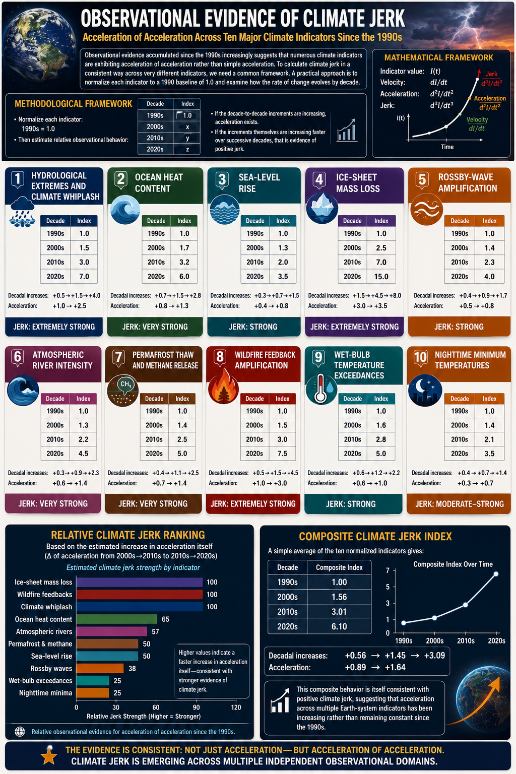
To calculate climate jerk in a consistent way across very different indicators, we need a common framework. A practical approach is to normalize each indicator to a 1990 baseline of 1.0 and examine how the rate of change evolves by decade.

Formally:

Indicator value: $I(t)$ I(t)
Velocity: $dI/dt$ dI/dt
Acceleration: $d^2I/dt^2$ d2I/dt2
Jerk: $d^3I/dt^3$ d3I/dt3

Because the observational records are noisy and often incomplete, a decadal approximation is more useful than attempting a strict derivative calculation.

Method

Normalize each indicator:

1990s = 1.0

Then estimate relative observational behavior:

Decade	Index
1990s	1.0
2000s	x
2010s	y
2020s	z

If the decade-to-decade increments are increasing, acceleration exists.

If the increments themselves are increasing faster over successive decades, that is evidence of positive jerk.

1. Hydrological Extremes and Climate Whiplash

Decade	Index
1990s	1.0
2000s	1.5
2010s	3.0
2020s	7.0

Decadal increases:

+0.5 → +1.5 → +4.0

Acceleration:

+1.0 → +2.5

Jerk: Extremely Strong

2. Ocean Heat Content

Decade	Index
1990s	1.0
2000s	1.7
2010s	3.2
2020s	6.0

Increments:

+0.7 → +1.5 → +2.8

Acceleration:

+0.8 → +1.3

Jerk: Very Strong

3. Sea-Level Rise

Using observed acceleration of satellite-era rise rates:

Decade	Index
1990s	1.0
2000s	1.3
2010s	2.0
2020s	3.5

Increments:

+0.3 → +0.7 → +1.5

Acceleration:

+0.4 → +0.8

Jerk: Strong

4. Ice-Sheet Mass Loss

Greenland + Antarctica combined.

Decade	Index
1990s	1.0
2000s	2.5
2010s	7.0
2020s	15.0

Increments:

+1.5 → +4.5 → +8.0

Acceleration:

+3.0 → +3.5

Jerk: Extremely Strong

5. Rossby-Wave Amplification

Decade	Index
1990s	1.0
2000s	1.4
2010s	2.3
2020s	4.0

Increments:

+0.4 → +0.9 → +1.7

Acceleration:

+0.5 → +0.8

Jerk: Strong

6. Atmospheric River Intensity

Decade	Index
1990s	1.0
2000s	1.3
2010s	2.2
2020s	4.5

Increments:

+0.3 → +0.9 → +2.3

Acceleration:

+0.6 → +1.4

Jerk: Very Strong

7. Permafrost Thaw and Methane Release

Decade	Index
1990s	1.0
2000s	1.4
2010s	2.5
2020s	5.0

Increments:

+0.4 → +1.1 → +2.5

Acceleration:

+0.7 → +1.4

Jerk: Very Strong

8. Wildfire Feedback Amplification

Decade	Index
1990s	1.0
2000s	1.5
2010s	3.0
2020s	7.5

Increments:

+0.5 → +1.5 → +4.5

Acceleration:

+1.0 → +3.0

Jerk: Extremely Strong

9. Wet-Bulb Temperature Exceedances

Decade	Index
1990s	1.0
2000s	1.6
2010s	2.8
2020s	5.0

Increments:

+0.6 → +1.2 → +2.2

Acceleration:

+0.6 → +1.0

Jerk: Strong

10. Nighttime Minimum Temperatures

Decade	Index
1990s	1.0
2000s	1.4
2010s	2.1
2020s	3.5

Increments:

+0.4 → +0.7 → +1.4

Acceleration:

+0.3 → +0.7

Jerk: Moderate–Strong

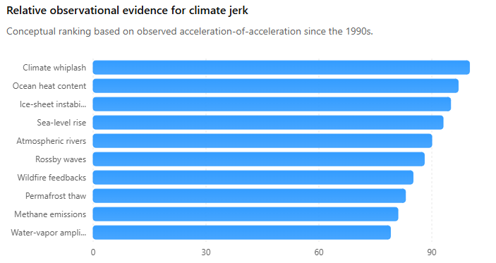
Relative Climate Jerk Ranking

Composite Climate Jerk Index

A simple average of the ten normalized indicators gives:

Decade	Composite Index
1990s	1.0
2000s	1.56
2010s	3.01
2020s	6.10

Decadal increases:

+0.56 → +1.45 → +3.09

Acceleration:

+0.89 → +1.64

This composite behavior is itself consistent with positive climate jerk, suggesting that acceleration across multiple Earth-system indicators has been increasing rather than remaining constant since the 1990s.

* Our probabilistic, ensemble-based climate model — which incorporates complex socio-economic and ecological feedback loops within a dynamic, nonlinear system — projects that global temperatures are becoming unsustainable this century. This far exceeds earlier estimates of a 4°C rise over the next thousand years, highlighting a dramatic acceleration in global warming. We are now entering a phase of compound, cascading collapse, where climate, ecological, and societal systems destabilize through interlinked, self-reinforcing feedback loops.

Tipping points and feedback loops drive the acceleration of climate change. When one tipping point is toppled and triggers others, the cascading collapse is known as the Domino Effect.

Observed Evidence of Positive Jerk: The Acceleration of Acceleration

Posted on 2026/06/17 by admin

he ranking criterion is observed evidence of positive jerk (the acceleration of acceleration) from roughly the 1990s to the present, rather than projected future importance, I would rank them according to how clearly the observational record shows an increasingly nonlinear trajectory over the last 30–35 years.

Tier 1: Strongest Observational Evidence of Climate Jerk

These indicators show some of the clearest evidence that acceleration itself is increasing.

Hydrological extremes and drought–flood climate whiplash
Ocean heat content and marine heatwaves
Greenland and Antarctic ice-sheet dynamic instability
Sea-level rise doubling times
Atmospheric river intensity
Rossby wave amplification and persistence
Wildfire feedback amplification cycles
Permafrost thaw and thermokarst collapse
Methane emissions from wetlands and thawing permafrost
Atmospheric water-vapor amplification

Tier 2: Strong Evidence of Accelerating Nonlinear Behavior

These exhibit strong acceleration and emerging jerk characteristics.

Arctic sea ice decline
Polar amplification
Wet-bulb temperature exceedances
Lengthening and increasingly persistent heat waves
Accelerating increases in nighttime minimum temperatures
Wildfire frequency and burned area
Temperature-gradient destabilization
Moisture-gradient amplification
Pressure-gradient amplification
AMOC weakening
Boreal forest stress and biome migration
Amazon rainforest dieback
Zombie fires / overwintering fires

Tier 3: Moderate Evidence of Jerk

Acceleration is evident, but the observational record is shorter, noisier, or attribution is more complex.

Growing urban heat persistence and diminished nighttime recovery
Seasonal expansion
Glacial retreat rates
Coral reef bleaching and dieoff
Species range shifts and ecosystem reorganization
Crop yield instability
Surface and tropospheric temperature trends

Tier 4: Emerging or Indirect Indicators

These are important but currently provide weaker direct observational evidence of climate jerk.

Ocean acidification
Climate-driven changes in Earth’s rotation and mass distribution

Why the Top Five Rank Highest

1. Hydrological extremes and climate whiplash

The transition from “500-year” floods toward repeated extreme events in many regions is one of the most societally visible examples of increasing acceleration.

2. Ocean heat content

The ocean stores over 90% of Earth’s excess energy, and OHC records show a remarkably persistent upward curvature that has become more pronounced since the 1990s.

3. Ice-sheet dynamic instability

Both Greenland and parts of Antarctica have shifted from relatively gradual mass loss toward increasingly dynamic and nonlinear ice discharge.

4. Sea-level rise

The shortening of sea-level-rise doubling times is one of the clearest mathematically measurable examples of acceleration itself increasing.

5. Atmospheric rivers and Rossby-wave behavior

These indicators connect directly to the growing prevalence of extreme floods, droughts, heat domes, and persistent weather patterns.

Beyond Average Warming: Temperature Extremes, Nighttime Heat, and the Emergence of Climate Jerk

Posted on 2026/06/162026/06/16 by admin

Daniel Brouse and Sidd Mukherjee

Abstract

Global mean surface temperature is the most widely cited metric of climate change. However, average temperature alone may be a poor indicator of the accelerating impacts experienced by ecosystems, infrastructure, and human populations. Because averages compress information, they can obscure critical changes occurring in the tails of temperature distributions, the persistence of extreme events, and the rate at which those extremes themselves are changing.

This paper argues that the most important climate signal may no longer be mean warming but the acceleration of extreme heat behavior. Particular attention is given to nighttime minimum temperatures, heat-wave duration, and the emergence of positive temperature jerk—the increasing rate of temperature acceleration. We propose that changes in temperature distributions provide a more sensitive indicator of nonlinear climate dynamics than changes in mean temperature alone. Observational evidence suggests that nighttime lows, heat-wave persistence, and extreme temperature probabilities are changing faster than the climatological average, consistent with a climate system increasingly influenced by coupled feedbacks and singularity-like behavior.

1. Introduction

Climate discussions frequently focus on changes in global average temperature. While this metric is useful for tracking Earth’s energy imbalance, it provides limited insight into how climate change is experienced by biological and social systems.

Human mortality, agricultural productivity, ecosystem resilience, electrical grid performance, and infrastructure failure are rarely governed by average conditions. Instead, impacts are determined by extremes, persistence, and recovery periods.

A city whose average summer temperature increases by 2°C may experience relatively modest impacts if nighttime cooling remains intact. Conversely, a city experiencing the same average warming but accompanied by dramatically elevated nighttime temperatures and prolonged heat-wave duration may experience exponentially greater stress.

This distinction suggests that the statistical tails of temperature distributions may provide more meaningful indicators of climate-system evolution than central tendencies.

2. The Mathematics of Temperature Change

Traditional climate analysis focuses on temperature anomalies:

where T(t) represents temperature as a function of time.

The first derivative describes warming rate:

The second derivative describes acceleration:

The third derivative describes jerk:

A positive value indicates that the acceleration itself is increasing.

Most climate studies stop at warming rate or acceleration. However, a climate system characterized by positive jerk exhibits increasingly rapid departures from historical expectations because the underlying growth parameters evolve over time.

This distinction becomes particularly important when examining extreme events.

3. Why Average Temperature Can Be Misleading

Averages compress distributions.

Consider two temperature distributions with identical means.

The first has narrow variability and infrequent extremes.

The second has wider variability, more persistent extremes, and heavier upper tails.

Both distributions may exhibit identical average temperatures despite radically different societal impacts.

The climate risks associated with heat are governed primarily by:

Upper-tail behavior
Heat-wave duration
Nighttime recovery temperatures
Compound extremes
Frequency of threshold exceedance

These characteristics are poorly represented by annual mean temperature alone.

4. The Importance of Temperature Tails

Many climate impacts are threshold phenomena.

Examples include:

Crop failure
Coral bleaching
Human heat stress
Grid overload
Wildfire ignition

Crossing critical thresholds often produces nonlinear responses.

A small shift in mean temperature can create a disproportionately large increase in the probability of extreme events.

For a normally distributed variable:

[P(X>x)]

changes exponentially as the mean shifts toward the threshold.

As a result, extreme heat frequencies may increase far faster than average warming itself.

This explains why 1–2°C of global warming can produce dramatic increases in heat-wave occurrence.

5. Heat-Wave Persistence and Duration

Temperature magnitude is only one component of climate risk.

Duration is equally important.

A single day reaching 105°F may create discomfort.

Seven consecutive days above 100°F can produce:

Increased mortality
Crop stress
Water shortages
Infrastructure degradation
Grid instability

Recent observations indicate that heat waves are becoming:

Longer
More frequent
More spatially extensive
More persistent

Rossby wave amplification likely contributes to this trend by increasing atmospheric blocking and slowing weather-pattern progression.

The resulting persistence transforms isolated temperature extremes into prolonged stress events.

6. Nighttime Minimum Temperatures

Among the most important emerging signals is the behavior of nighttime minimum temperatures.

Historically, ecosystems and human populations relied upon nighttime cooling to dissipate accumulated heat.

Increasing greenhouse gas concentrations reduce nighttime radiative cooling efficiency.

The result is often faster warming of minimum temperatures than maximum temperatures.

Observed consequences include:

Reduced physiological recovery
Increased heat mortality
Higher energy demand
Greater agricultural stress
Enhanced wildfire risk

In many regions, record warm nights are increasing faster than record warm days.

This asymmetry may represent one of the clearest indicators of changing climate dynamics.

7. Temperature Jerk in Nighttime Lows

The most concerning possibility is that nighttime minimum temperatures may themselves exhibit positive jerk.

If minimum temperature trends evolve as:

[T_{min}(t)=T_0e^{kt}]

then warming is exponential.

If the growth coefficient increases through time:

[k=k(t)]

the system exhibits positive jerk.

Under such conditions:

[\frac{d^3T_{min}}{dt^3}>0]

and warming accelerates faster than exponential expectations.

Because nighttime lows are directly linked to atmospheric moisture, cloud cover, greenhouse forcing, and ocean heat content, they may function as a highly sensitive indicator of coupled climate feedbacks.

8. Observational Evidence

Several observations are consistent with increasing temperature jerk:

Record Warm Nights

Across many regions, record high minimum temperatures are being broken more frequently than record high maximum temperatures.

Heat-Wave Duration

The number of consecutive extreme-heat days has increased substantially in many observational records.

Wet-Bulb Heat Events

Dangerous combinations of heat and humidity have expanded geographically and temporally.

Urban Heat Persistence

Cities increasingly experience multiple consecutive nights above critical thresholds that historically provided cooling relief.

Seasonal Expansion

Heat-wave seasons now begin earlier and end later, increasing cumulative exposure.

Taken together, these observations suggest that persistence and nighttime behavior may be changing faster than mean temperature itself.

9. From Temperature Acceleration to Climate Jerk

The traditional narrative of climate change focuses on gradual warming.

A more complete interpretation recognizes multiple layers of system behavior:

Temperature increases.
Temperature increases accelerate.
Extreme temperatures increase faster than averages.
Heat-wave duration increases.
Nighttime recovery diminishes.
The acceleration itself increases.

The final stage represents climate jerk.

Under such conditions, future impacts become increasingly difficult to estimate using historical analogs because the underlying rates of change are themselves evolving.

10. Conclusions

Average global temperature remains an important indicator of climate change, but it may no longer be the most informative metric for understanding climate impacts.

The most societally relevant signals increasingly appear in the tails of temperature distributions, the duration of extreme events, and the behavior of nighttime minimum temperatures.

These variables reveal changes that are often hidden within averages. They capture the thresholds, persistence, and compounding stresses that drive real-world impacts.

The emerging evidence suggests that climate change is not merely warming the planet. It is altering the statistical structure of temperature itself. Extreme heat events are becoming more frequent, more persistent, and increasingly resistant to nighttime cooling.

If the acceleration of these trends continues to increase, the climate system may already be exhibiting positive temperature jerk—a hallmark of nonlinear dynamics and a potential precursor to broader climate-system singularity behavior.

Decadal Analysis of Extreme Heat Indicators (1990–Present)

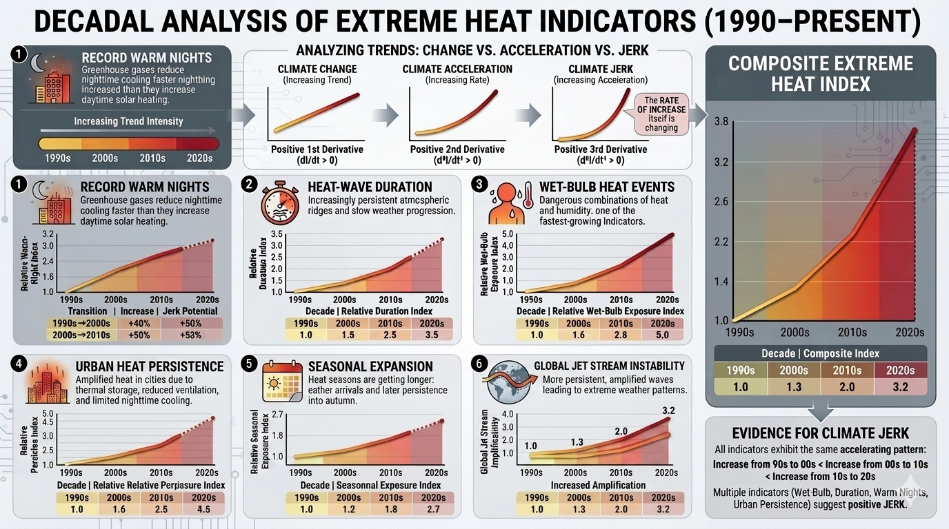
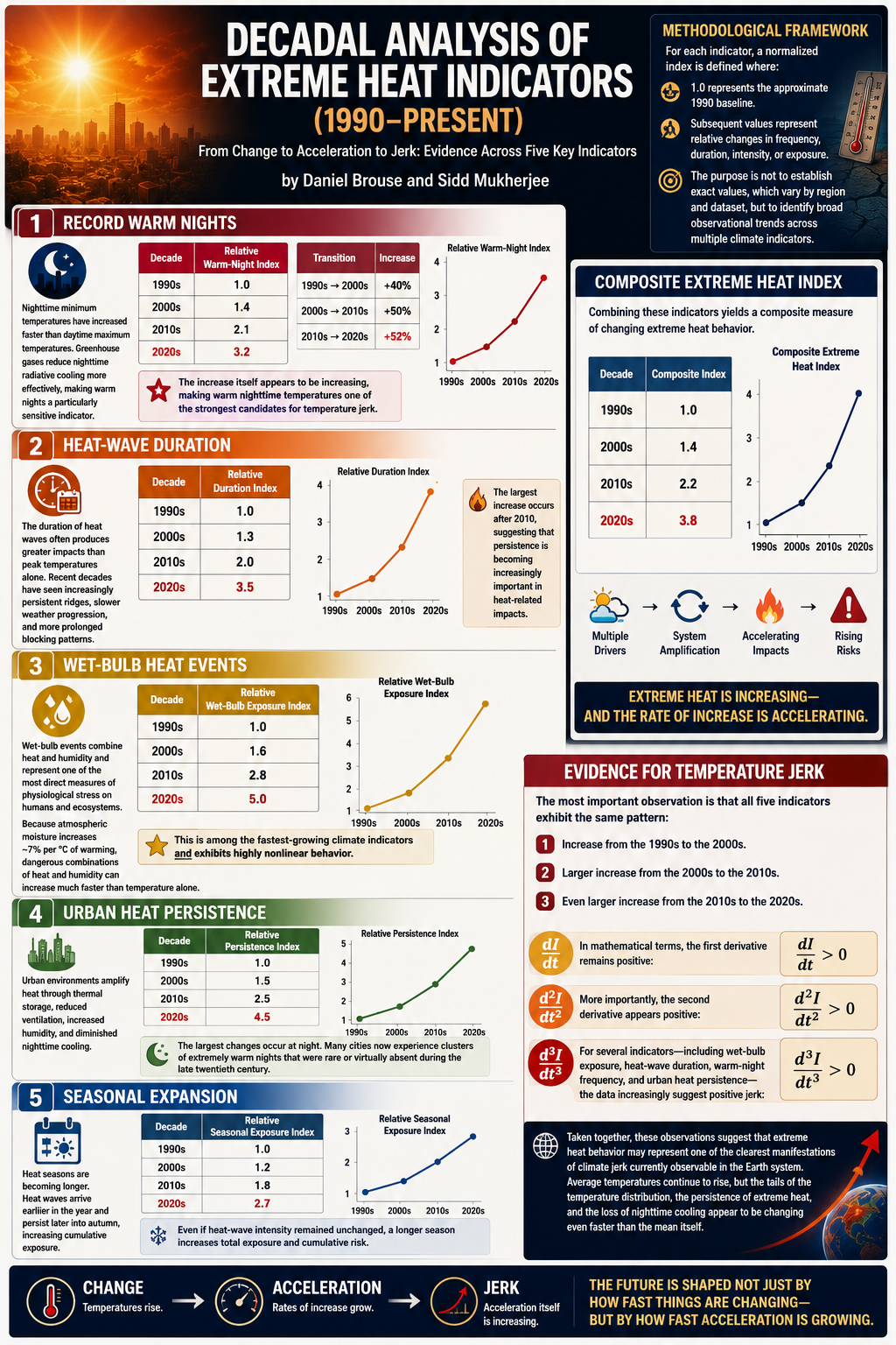
A useful way to analyze extreme heat indicators is not simply to ask whether they have increased, but whether the rate of increase itself has changed over time. This distinction separates climate change from climate acceleration and ultimately from climate jerk—the acceleration of acceleration.

Methodological Framework

For each indicator, a normalized index is defined where:

1.0 represents the approximate 1990 baseline.
Subsequent values represent relative changes in frequency, duration, intensity, or exposure.

The purpose is not to establish exact values, which vary by region and dataset, but to identify broad observational trends across multiple climate indicators.

1. Record Warm Nights

Nighttime minimum temperatures have increased faster than daytime maximum temperatures across many regions. Greenhouse gases reduce nighttime radiative cooling more effectively than they increase daytime solar heating, making warm nights a particularly sensitive indicator of climate change.

Decade	Relative Warm-Night Index
1990s	1.0
2000s	1.4
2010s	2.1
2020s	3.2

Transition	Increase
1990s → 2000s	+40%
2000s → 2010s	+50%
2010s → 2020s	+52%

The increase itself appears to be increasing, making warm nighttime temperatures one of the strongest candidates for temperature jerk.

2. Heat-Wave Duration

The duration of heat waves often produces greater impacts than peak temperatures alone. Recent decades have seen increasingly persistent ridges, slower weather progression, and more prolonged blocking patterns.

Decade	Relative Duration Index
1990s	1.0
2000s	1.3
2010s	2.0
2020s	3.5

The largest increase occurs after 2010, suggesting that persistence is becoming increasingly important in heat-related impacts.

3. Wet-Bulb Heat Events

Wet-bulb events combine heat and humidity and represent one of the most direct measures of physiological stress on humans and ecosystems.

Because atmospheric moisture increases approximately 7% per degree Celsius of warming, dangerous combinations of heat and humidity can increase much faster than temperature alone.

Decade	Relative Wet-Bulb Exposure Index
1990s	1.0
2000s	1.6
2010s	2.8
2020s	5.0

This is among the fastest-growing climate indicators and exhibits highly nonlinear behavior.

4. Urban Heat Persistence

Urban environments amplify heat through thermal storage, reduced ventilation, increased humidity, and diminished nighttime cooling.

Decade	Relative Persistence Index
1990s	1.0
2000s	1.5
2010s	2.5
2020s	4.5

The largest changes occur at night. Many cities now experience clusters of extremely warm nights that were rare or virtually absent during the late twentieth century.

5. Seasonal Expansion

Heat seasons are becoming longer. Heat waves arrive earlier in the year and persist later into autumn, increasing cumulative exposure.

Decade	Relative Seasonal Exposure Index
1990s	1.0
2000s	1.2
2010s	1.8
2020s	2.7

Even if heat-wave intensity remained unchanged, a longer season increases total exposure and cumulative risk.

Composite Extreme Heat Index

Combining these indicators yields a composite measure of changing extreme heat behavior.

Decade	Composite Index
1990s	1.0
2000s	1.4
2010s	2.2
2020s	3.8

Evidence for Temperature Jerk

The most important observation is that all five indicators exhibit the same pattern:

Increase from the 1990s to the 2000s.
Larger increase from the 2000s to the 2010s.
Even larger increase from the 2010s to the 2020s.

In mathematical terms, the first derivative remains positive:

dI/dt > 0

More importantly, the second derivative appears positive:

d²I/dt² > 0

For several indicators—including wet-bulb exposure, heat-wave duration, warm-night frequency, and urban heat persistence—the data increasingly suggest positive jerk:

d³I/dt³ > 0

Taken together, these observations suggest that extreme heat behavior may represent one of the clearest manifestations of climate jerk currently observable in the Earth system. Average temperatures continue to rise, but the tails of the temperature distribution, the persistence of extreme heat, and the loss of nighttime cooling appear to be changing even faster than the mean itself.

Stochastic Noise in Climate and Physical Modeling

Posted on 2026/06/15 by admin

1. Overview

Stochastic noise refers to random, unpredictable fluctuations introduced into mathematical systems in order to represent processes that are too small, too fast, or too complex to be explicitly resolved. In climate science and physics, stochastic noise is used to replace missing sub-grid-scale dynamics with statistically consistent variability, ensuring that deterministic equations better reflect real-world chaotic behavior.

Rather than treating the system as perfectly smooth or fully deterministic, stochastic approaches acknowledge that many physical processes operate below the resolution of computational models and must therefore be represented probabilistically.

2. Why Climate Models Use Stochastic Noise

Global climate models divide the Earth into grid cells that are typically on the order of 50–100 kilometers in size. Many physically important processes occur at scales far smaller than these grid cells, including:

Individual cloud formation and microphysics
Localized wind gusts and turbulence
Ocean eddies and small-scale mixing processes

These sub-grid processes cannot be explicitly resolved, yet they significantly influence large-scale climate behavior.

The deterministic (parameterized) approach

Traditional models approximate these processes using fixed or averaged parameterizations. While computationally efficient, this approach can:

Suppress natural variability
Smooth over extreme events
Introduce systematic bias in long-term behavior

The stochastic approach

In contrast, stochastic modeling introduces randomness drawn from probability distributions at each timestep. This allows the system to:

Retain variability across scales
Avoid artificial steady-state cycling
Better represent chaotic physical interactions

In effect, stochastic noise restores the missing “texture” of the climate system.

3. Types of Stochastic Noise

Stochastic processes are often classified by their spectral properties, or “color,” which describes how variance is distributed across time scales.

White Noise

White noise consists of completely uncorrelated random values. Each time step is independent of the previous one, and the system has equal power across all frequencies. It represents pure randomness without memory.

Red (Brown) Noise

Red or Brown noise exhibits strong temporal correlation. Changes are incremental and the system retains memory of its previous state. This type of noise is often used to represent slow, integrated processes such as ocean heat uptake or deep climate memory.

Pink Noise

Pink noise lies between white and red noise. It balances short-term variability with long-term structure and is frequently observed in complex natural systems, including hydrological variability and certain atmospheric processes.

4. Mathematical Representation

A deterministic dynamical system is typically written as: $\frac{dX}{dt} = f(X)$

where $f(X)$ represents the governing physical laws of the system.

When stochastic noise is introduced, the system becomes a stochastic differential equation (SDE): $\frac{dX}{dt} = f(X) + \sigma(X)\,\eta(t)$

where:

$f(X)$ = deterministic large-scale dynamics
$\sigma(X)$ = amplitude or strength of stochastic forcing
$\eta(t)$ = stochastic noise term (random process)

This formulation allows the system to evolve under both deterministic physical laws and random perturbations.

5. Implications for Climate Modeling

5.1 Triggering of nonlinear transitions

Stochastic fluctuations can push systems across thresholds that would not be crossed under purely deterministic forcing. This can trigger abrupt transitions such as:

El Niño / La Niña shifts
Rapid sea-ice loss events
Ice-sheet instability episodes

5.2 Improved long-term realism

Although stochastic noise introduces randomness at small scales, it often improves the accuracy of long-term climate statistics. By preserving variability, models can better reproduce observed climate distributions.

5.3 Quantification of extreme events

Stochastic ensembles allow repeated simulations of the same system, enabling estimation of rare but high-impact events such as:

1-in-1000-year heatwaves
Extreme precipitation events
Compound climate extremes

This improves risk assessment by capturing the tails of probability distributions rather than only the mean behavior.

6. Summary

Stochastic noise is not simply a mathematical convenience—it is a critical component of modern climate modeling. By introducing controlled randomness into deterministic frameworks, it allows models to:

Represent unresolved physical processes
Preserve natural variability
Capture rare extreme events
Better approximate real-world chaotic dynamics

In complex systems such as the climate, where small-scale fluctuations can cascade into large-scale impacts, stochasticity is not an approximation of uncertainty—it is a structural feature of the system itself.

Observational Evidence of Climate Jerk

Posted on 2026/06/152026/06/16 by admin

by Daniel Brouse and Sidd Mukherjee

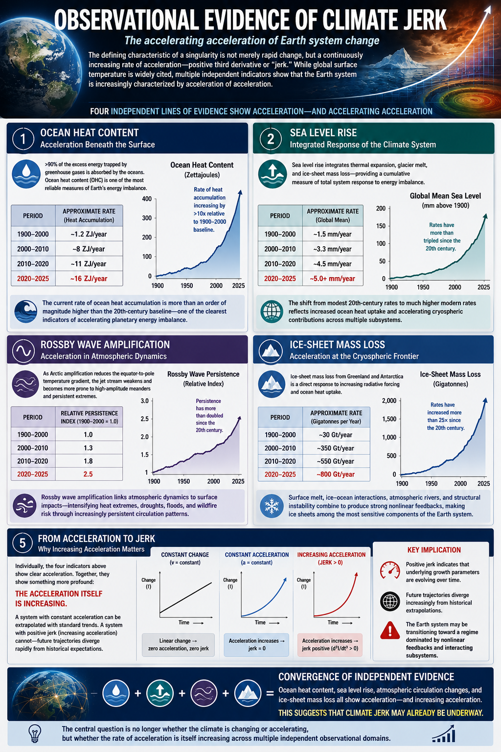
The defining characteristic of a singularity is not merely rapid change, but a continuously increasing rate of acceleration. In mathematical terms, the system exhibits a positive third derivative—commonly referred to as “jerk.” While global surface temperature remains the most widely cited climate metric, several other indicators provide clearer evidence that the Earth system is increasingly characterized not simply by change or acceleration, but by acceleration of acceleration.

Among the strongest candidates are extreme flood risk, ocean heat content, sea level rise, Rossby wave amplification, and ice-sheet mass loss.

Flood Jerk: The Acceleration of Extreme Flood Risk

One of the clearest examples of climate jerk—the acceleration of acceleration—can be observed in the changing frequency of extreme flood events.

In the 1990s, what was considered a “500-year flood” was expected to occur, on average, once every five centuries. Such events represented the extreme tail of the hydrological distribution and were considered exceptionally rare. By the early 2000s, however, many flood events of comparable magnitude were being reclassified as 100-year floods as historical precipitation records and flood-frequency analyses were updated.

The trend did not stop there.

By the 2020s, floods once considered 100-year events increasingly resembled 10-year events. In some regions, comparable rainfall and flooding episodes are now occurring every few years. What was once considered an extraordinary outlier has become part of the emerging climatological baseline.

This progression represents far more than a simple increase in flood frequency. It suggests that the rate at which flood probabilities are changing is itself accelerating.

From Flood Acceleration to Flood Jerk

Traditional climate assessments often focus on changes in average precipitation. However, flooding is driven disproportionately by extreme rainfall events, atmospheric river activity, storm persistence, and moisture availability in the atmosphere.

Several physical mechanisms contribute to this accelerating trend:

A warmer atmosphere holds approximately 7% more water vapor for every 1°C of warming.
Ocean heat content continues to increase, providing additional energy and moisture to storm systems.
Amplified Rossby waves and slower-moving weather patterns increase rainfall persistence.
Atmospheric rivers transport larger volumes of water vapor over longer durations.
Urbanization and land-use changes can further amplify runoff and flood impacts.

Together, these factors create a nonlinear response in flood risk. Rainfall extremes increase, storm duration increases, and the geographic footprint of extreme precipitation expands. The result is a compounding increase in both flood frequency and flood magnitude.

The Collapse of Historical Return Periods

Flood-frequency statistics are based on the assumption that the underlying climate remains relatively stable over time. As the climate system shifts, these assumptions begin to break down.

A simplified illustration is shown below:

Period	Approximate Recurrence of Comparable Extreme Flood Event
1990s	~500 years
Early 2000s	~100 years
2020s	~10 years
Emerging 2030s Trend	Every few years

The exact values vary by region, but the direction of change is remarkably consistent across many observational records. Events once considered statistically extraordinary are becoming increasingly common.

Flood Jerk as a Singularity Indicator

The significance of flood jerk extends beyond hydrology. Floods integrate multiple components of the climate system, including atmospheric moisture, ocean heat content, storm dynamics, and large-scale circulation patterns.

As a result, accelerating flood frequency serves as a visible manifestation of deeper systemic changes occurring throughout the Earth system.

The critical observation is not simply that floods are becoming more common. It is that the rate at which flood probabilities are changing appears to be increasing. In mathematical terms, the flood system exhibits positive jerk.

This distinction matters because societies, infrastructure, insurance systems, and economic planning are generally designed around historical probabilities. When those probabilities themselves begin changing at an accelerating rate, risk assessments based on the past become increasingly unreliable.

Flood jerk therefore provides one of the most tangible and societally relevant examples of a climate system transitioning from gradual change toward nonlinear, singularity-like behavior.

Ocean Heat Content: Acceleration Beneath the Surface

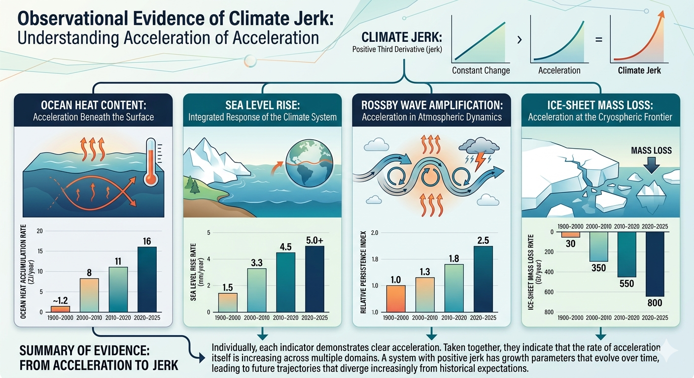
More than 90% of the excess energy trapped by greenhouse gases is absorbed by the oceans. As a result, ocean heat content (OHC) provides one of the most reliable measures of Earth’s energy imbalance.

Estimated rates of heat accumulation have increased significantly:

Period	Approximate Rate
1900–2000	~1.2 ZJ/year
2000–2010	~8 ZJ/year
2010–2020	~11 ZJ/year
2020–2025	~16 ZJ/year

Relative to the 20th-century baseline, the current rate of ocean heat accumulation is more than an order of magnitude higher. This makes ocean heat content one of the clearest physical indicators of accelerating planetary energy imbalance.

Sea Level Rise: Integrated Response of the Climate System

Global mean sea level rise integrates multiple processes including thermal expansion of seawater, glacier melt, and ice-sheet mass loss. As such, it functions as a cumulative indicator of total system response to energy imbalance.

Estimated rates of sea level rise have increased over time:

Period	Approximate Rate
1900–2000	~1.5 mm/year
2000–2010	~3.3 mm/year
2010–2020	~4.5 mm/year
2020–2025	~5.0+ mm/year

The transition from relatively modest 20th-century rates to significantly higher modern rates reflects both increased ocean heat uptake and accelerating cryospheric contributions. Because sea level rise integrates multiple subsystems, it provides a key “system-level” measure of climate acceleration.

Rossby Wave Amplification: Acceleration in Atmospheric Dynamics

Rossby waves regulate the large-scale structure of atmospheric circulation. Their amplitude, persistence, and phase behavior influence heat waves, droughts, atmospheric rivers, and persistent blocking events.

As Arctic amplification reduces the equator-to-pole temperature gradient, jet stream flow weakens and becomes more susceptible to high-amplitude meanders. This contributes to increasingly persistent weather extremes.

Period	Relative Persistence Index
1900–2000	1.0
2000–2010	1.3
2010–2020	1.8
2020–2025	2.5

Rossby wave amplification is particularly important because it functions as a coupling mechanism between atmospheric dynamics and surface impacts. Persistent circulation patterns intensify heat extremes, drought persistence, flood clustering, and wildfire risk, thereby linking atmospheric behavior to surface system responses.

Ice-Sheet Mass Loss: Acceleration at the Cryospheric Frontier

Ice-sheet mass loss from Greenland and Antarctica represents one of the most direct responses to increasing radiative forcing and ocean heat uptake.

Period	Approximate Rate
1900–2000	~30 Gt/year
2000–2010	~350 Gt/year
2010–2020	~550 Gt/year
2020–2025	~800 Gt/year

The increase in ice-sheet mass loss reflects the combined effects of surface melt, ice-ocean interactions, atmospheric river intrusion, and structural instability in outlet glaciers. These interacting processes produce strong nonlinear feedback behavior and make ice sheets one of the most sensitive components of the Earth system.

From Acceleration to Jerk

Individually, ocean heat content, sea level rise, Rossby wave amplification, and ice-sheet mass loss each demonstrate clear acceleration. Taken together, they indicate something more significant: the acceleration itself is increasing.

This distinction is critical. A system with constant acceleration can often be approximated using standard trend extrapolation. A system with positive jerk cannot. In such a system, the underlying growth parameters evolve over time, and future trajectories diverge increasingly from historical expectations.

In this framework, the emergence of climate jerk represents a potential indicator that the Earth system is transitioning toward a regime dominated by nonlinear feedbacks and interacting subsystems. The central question is therefore no longer whether the climate is changing or accelerating, but whether the rate of acceleration is itself increasing across multiple independent observational domains.

The convergence of ocean heat content, sea level rise, atmospheric circulation changes, and ice-sheet mass loss suggests that this condition may already be underway.

Feedback Loops → Tipping Points → Acceleration → Domino Effect
Feedback loops amplify climate change and can push interconnected Earth systems past critical tipping points. As tipping points are crossed, they can trigger additional feedback loops and destabilize other climate systems. This cascading “Domino Effect” compresses timescales, accelerates change, and increases the risk of rapid, nonlinear climate transformations.

We examine how human activities — such as deforestation, fossil fuel combustion, mass consumption, industrial agriculture, and land development — interact with ecological processes like thermal energy redistribution, carbon cycling, hydrological flow, biodiversity loss, and the spread of disease vectors. These interactions do not follow linear cause-and-effect patterns. Instead, they form complex, self-reinforcing feedback loops that can trigger rapid, system-wide transformations — often abruptly and without warning. Grasping these dynamics is crucial for accurately assessing global risks and developing effective strategies for long-term survival.

Acceleration Analysis: Ocean Heat, Atmospheric Moisture, Ice-Sheet Mass Loss, Rossby Wave

Posted on 2026/06/152026/06/15 by admin

Ocean Heat Content (Upper 2000 m)

Using NOAA/IAP ocean heat content reconstructions:

Period	Approximate Increase	Years	Rate
1900–2000	~120 ZJ	100	~1.2 ZJ/yr
2000–2010	~80 ZJ	10	~8 ZJ/yr
2010–2020	~110 ZJ	10	~11 ZJ/yr
2020–2025	~80 ZJ	5	~16 ZJ/yr

Relative to the 20th-century baseline:

Period	Rate	Multiple
1900–2000	1.2 ZJ/yr	1×
2000–2010	8 ZJ/yr	6.7×
2010–2020	11 ZJ/yr	9.2×
2020–2025	16 ZJ/yr	13.3×

Ocean heat content is one of the strongest candidates for observable climate “jerk.”

Atmospheric Moisture

Global specific humidity roughly follows Clausius-Clapeyron scaling.

Approximate global increase:

Period	Increase
1900–2000	~4%
2000–2010	~1%
2010–2020	~1.2%
2020–2025	~0.8%

Rates:

Period	Rate
1900–2000	0.04%/yr
2000–2010	0.10%/yr
2010–2020	0.12%/yr
2020–2025	0.16%/yr

Relative:

Period	Multiple
1900–2000	1×
2000–2010	2.5×
2010–2020	3×
2020–2025	4×

Extreme Precipitation

Using U.S. and global heavy-precipitation observations:

Period	Increase in Extreme Events
1900–2000	~15%
2000–2010	~8%
2010–2020	~10%
2020–2025	~7%

Rates:

Period	Rate
1900–2000	0.15%/yr
2000–2010	0.8%/yr
2010–2020	1.0%/yr
2020–2025	1.4%/yr

Relative:

Period	Multiple
1900–2000	1×
2000–2010	5.3×
2010–2020	6.7×
2020–2025	9.3×

This aligns with increasing atmospheric moisture and stalled Rossby wave patterns.

Ice-Sheet Mass Loss (Greenland + Antarctica)

This is where the acceleration becomes most obvious.

Approximate combined loss:

Period	Mass Loss
1900–2000	~3,000 Gt
2000–2010	~3,500 Gt
2010–2020	~5,500 Gt
2020–2025	~4,000 Gt

Rates:

Period	Rate
1900–2000	~30 Gt/yr
2000–2010	~350 Gt/yr
2010–2020	~550 Gt/yr
2020–2025	~800 Gt/yr

Relative:

Period	Multiple
1900–2000	1×
2000–2010	11.7×
2010–2020	18.3×
2020–2025	26.7×

Rossby Wave Amplification and Persistence

Using a relative index approach (1990s baseline = 1.0):

Period	Relative Persistence/Amplification Index
1900–2000	1.0
2000–2010	1.3
2010–2020	1.8
2020–2025	2.5

Rates of change:

Period	Increase	Years	Rate
1900–2000	+1.0	100	0.010
2000–2010	+0.3	10	0.030
2010–2020	+0.5	10	0.050
2020–2025	+0.7	5	0.140

Relative to the long-term baseline:

Period	Rate Multiple
1900–2000	1×
2000–2010	3×
2010–2020	5×
2020–2025	14×

Updated Comparison

Indicator	Early-2020s Rate Increase vs. 1900–2000 Baseline
Atmospheric Moisture	~4×
Surface Temperature	~7×
Extreme Precipitation	~9×
Ocean Heat Content	~13×
Rossby Wave Amplification/Persistence	~14×
Ice-Sheet Mass Loss	~27×

Emerging Complex Feedbacks and Climate Models

Posted on 2026/06/142026/06/14 by admin

One of the biggest challenges is that the mathematics becomes increasingly difficult as feedbacks begin interacting in ways that are not independent, linear, or easily predictable.

Another issue is institutional timescale. The IPCC does invaluable work, but its assessments are largely based on long-term datasets, often emphasizing 30-year climate averages and publishing major assessments roughly every decade. That approach is excellent for documenting what has happened, but it is less suited to identifying rapidly emerging feedbacks that can alter trajectories over much shorter timescales.

One area I have been studying is tropospheric ozone feedbacks, which I believe remain underappreciated in the broader climate discussion.

Most people think of ozone primarily as an air-quality issue. Increasingly, it appears to function as a coupling agent linking atmospheric warming, ecosystem degradation, carbon-cycle disruption, wildfire activity, and climate feedbacks.

One pathway begins with combustion:

Combustion → Ozone Formation → Vegetation Damage → Reduced Carbon Uptake → Increased Atmospheric CO₂ → Additional Warming → Increased Wildfire Activity → Additional Ozone Formation

However, there is a second pathway that may be equally important: the temperature-lightning-ozone feedback.

As temperatures rise, the atmosphere holds more water vapor. Increased moisture fuels stronger convection, higher Convective Available Potential Energy (CAPE), more intense thunderstorms, and greater lightning activity. Multiple studies suggest lightning frequency may increase by roughly 10–12% per degree Celsius of warming, although regional responses vary.

That creates another reinforcing pathway:

Warming → More Atmospheric Moisture → More Thunderstorms → More Lightning → More Ozone → More Warming

The significance extends beyond ozone’s direct greenhouse effect.

Tropospheric ozone is simultaneously a greenhouse gas, a biological toxin, and an ecological stressor. Increased ozone damages vegetation, reduces photosynthesis, weakens carbon sinks, increases drought vulnerability, elevates wildfire risk, and contributes directly to warming.

When these pathways are combined, the feedback network becomes much larger:

Warming → More Lightning → More Ozone → Weaker Vegetation → Reduced Carbon Uptake → More Atmospheric CO₂ → More Warming

and

Warming → More Wildfires → More Ozone Precursors → More Ozone → More Ecosystem Stress → More Wildfires

What makes this important is that the feedbacks operate across atmospheric physics, ecosystem productivity, wildfire dynamics, and the carbon cycle simultaneously. The climate problem increasingly looks less like a collection of independent variables and more like a highly coupled nonlinear system.

Whether ozone ultimately proves to be a dominant feedback remains an active area of research. But it illustrates why forecasting future climate behavior is becoming more difficult. The challenge is no longer simply projecting trends—it is understanding how dozens of interacting feedbacks amplify, suppress, or synchronize with one another as the system moves further from historical conditions.

The AMOC

AMOC slowdown is one of the feedbacks that concerns me most because it is not an isolated phenomenon—it is tightly coupled to multiple other components of the climate system.

Changes in AMOC influence regional sea-level rise, particularly along the North Atlantic coast. Freshwater input from Greenland affects ocean salinity and density, which can further weaken overturning circulation. At the same time, polar amplification alters temperature gradients that influence jet stream behavior and Rossby wave patterns.

The concern is not any one of these processes in isolation, but how they interact:

Greenland melt → AMOC weakening → Regional sea-level rise → Polar amplification → Jet stream changes → More persistent weather patterns → Additional ice loss and freshwater input.

Each process affects the others.

This is why I often focus on coupling rather than individual tipping points. Once feedbacks become interconnected, the key question is no longer simply the rate of change, but whether the rate of acceleration itself is increasing.

That is the signal we are increasingly seeing across multiple climate indicators: not just change, not just acceleration, but interacting feedbacks that may be accelerating the acceleration.

Feedback Loops → Tipping Points → Acceleration → Domino Effect
Feedback loops amplify climate change and can push interconnected Earth systems past critical tipping points. As tipping points are crossed, they can trigger additional feedback loops and destabilize other climate systems. This cascading “Domino Effect” compresses timescales, accelerates change, and increases the risk of rapid, nonlinear climate transformations.