The Climate Acceleration Index and Cross-Component Coherence in Ocean Heat Content, Sea Level, Marine Heatwaves, and Atmospheric Moisture

---

Executive Summary

The Earth’s climate system is undergoing a clear regime shift away from historically linear behavior toward accelerating nonlinear and compounding dynamics characterized by systematically shrinking effective doubling times.

Multiple independent Earth system indicators demonstrate synchronized acceleration, with converging evidence that growth rates are increasing across coupled components of the climate system.

Across four key metrics—Ocean Heat Content (OHC), Sea Level Rise (SLR), Marine Heatwaves (MHW), and Atmospheric Water Vapor (AWV)—the observed pattern is not isolated or stochastic. Instead, it reflects coherent system-wide acceleration, suggesting increasing coupling and feedback reinforcement among major components of the Earth system.

Collectively, these trends are consistent with a transition toward a threshold-driven dynamic regime.

Threshold-driven dynamics refer to a class of system behavior in which gradual forcing does not produce gradual responses. Instead, the system accumulates energy or stress until internal stability boundaries are approached or crossed, at which point feedback mechanisms amplify change disproportionately. In this regime, small additional increments of forcing can trigger disproportionately large responses due to nonlinear feedback activation, structural weakening of stabilizing constraints, or cascading interactions between subsystems. Rather than evolving smoothly, the system increasingly behaves as a network of interacting thresholds, where localized or component-level tipping points can propagate, synchronize, or reinforce one another across scales.

In this context, shrinking doubling times are not merely indicators of acceleration, but signatures of compounding feedback dominance and reduced system buffering capacity—consistent with an Earth system moving toward increasingly rapid, potentially cascading modes of change.

Introduction

Shrinking Doubling Times and the Transition Toward Instantaneous Growth in the Earth System

The Earth system is commonly described through long-term trends in temperature, ocean heat content, sea level, and extreme event frequency. These trends are typically represented using linear rates or, in some cases, stationary exponential growth assumptions. While useful for first-order characterization, these representations implicitly assume that the underlying growth dynamics of the system are time-invariant.

However, increasing observational evidence suggests that multiple components of the Earth system are not only changing in magnitude, but also in the rate at which they change. This distinction is critical: it implies that the Earth system may be transitioning from a regime of approximately stationary growth toward one characterized by non-stationary, time-dependent acceleration.

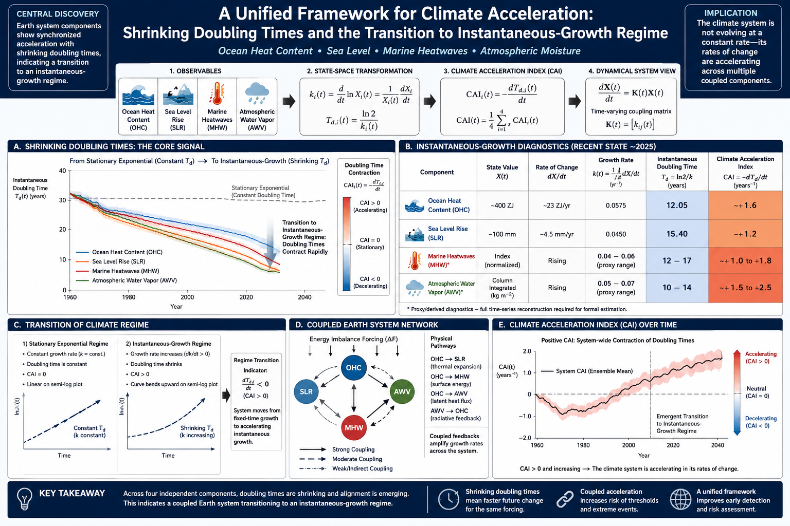
A key diagnostic for this transition is the instantaneous doubling time, defined as:$$T_d(t)=\frac{\ln 2}{k(t)}=\frac{\ln 2}{\frac{d}{dt}\ln X(t)}$$Td​(t)=k(t)ln2​=dtd​lnX(t)ln2​

where $X(t)$X(t) represents a climate state variable such as ocean heat content, sea level, or atmospheric moisture. Unlike traditional doubling-time estimates derived from fitted exponential trends, this formulation is fully time-local and does not assume stationarity in the growth rate.

Within this framework, the central question is not whether a variable is increasing, but whether the timescale of increase itself is changing over time.

If the effective growth rate $k(t)$k(t) increases, then the doubling time $T_d(t)$Td​(t) necessarily decreases. This leads to a fundamental diagnostic shift: the Earth system is no longer characterized by fixed exponential time constants, but by evolving temporal scales of change.

This behavior can be interpreted as a transition from:

• Trend-dominated dynamics, where rates are approximately constant
  to
• growth-rate dominated dynamics, where the rate of change itself evolves

In this latter regime, the system is more naturally described as a state-space process with time-dependent growth operators, rather than a static parametric model.

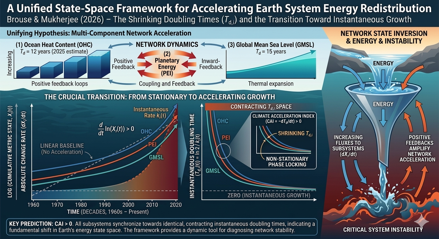
Recent observational reconstructions of ocean heat content, sea level rise, atmospheric moisture, and marine heat extremes suggest that these systems may exhibit partially synchronized changes in their instantaneous growth rates. This raises the possibility that Earth system components are not evolving independently, but are instead embedded in a coupled structure governed by a shared energy imbalance.

In this context, the concept of a Climate Acceleration Index (CAI) emerges as a reduced-order diagnostic of system-wide behavior, defined through the rate of contraction of doubling times:$$CAI(t) = -\frac{dT_d(t)}{dt}$$CAI(t)=−dtdTd​(t)​

A positive CAI indicates that the system is transitioning toward shorter characteristic growth timescales, consistent with accelerating dynamics in the underlying state variables.

This study develops and applies a unified framework for diagnosing these changes across multiple Earth system components. By transforming observables into instantaneous growth-rate space, we examine whether the climate system is best understood as a collection of independently evolving trends, or as a coupled dynamical system undergoing coordinated temporal acceleration.

The central hypothesis explored here is:

The Earth system is undergoing a regime transition in which growth processes are no longer characterized by stationary timescales, but by continuously evolving instantaneous doubling times reflecting nonlinear energy redistribution across coupled subsystems.

Abstract

We develop a unified state-space framework for diagnosing temporal changes in Earth system energy redistribution using a non-stationary growth-rate representation of key climate variables. Rather than analyzing trends in individual observables, we transform each variable into a logarithmic growth-rate space and define a shared diagnostic: the instantaneous doubling time and its rate of change.

We apply this framework to four coupled components of the Earth system: ocean heat content, global mean sea level, marine heatwave occurrence, and atmospheric water vapor. Each variable is expressed in terms of a time-dependent growth rate $k_i(t)$ki​(t), estimated from observational data using non-parametric smoothing and derivative reconstruction.

We define a unified diagnostic, the Climate Acceleration Index (CAI), as a first-order measure of the contraction rate of doubling times across system components. We further embed this formulation in a coupled dynamical systems representation:$$\frac{d\mathbf{X}}{dt} = \mathbf{K}(t)\mathbf{X}(t)$$dtdX​=K(t)X(t)

where $\mathbf{K}(t)$K(t) is a time-dependent interaction operator inferred from observational growth-rate fields.

We show that this representation provides a mathematically consistent framework for diagnosing synchronized non-stationarity across multiple components of the Earth system.

---

1. Introduction

The Earth system is commonly analyzed through independent trend estimates of physical variables such as ocean heat content (OHC), sea level rise (SLR), atmospheric moisture, and extreme event statistics. However, these variables are not independent; they are coupled through a shared energy imbalance and nonlinear feedback structure.

Traditional trend-based approaches implicitly assume either:

• stationary linear growth, or
• stationary exponential growth

Both assumptions impose time-invariant structure on a system that is physically coupled and potentially non-stationary.

We instead propose a growth-rate state-space formulation, where the primary object of analysis is not the variable itself, but its instantaneous logarithmic growth rate.

---

2. State-Space Formulation of Earth System Variables

We define a vector of Earth system observables:$$\mathbf{X}(t) = \begin{bmatrix} X_1(t) \\ X_2(t) \\ X_3(t) \\ X_4(t) \end{bmatrix} = \begin{bmatrix} \text{OHC}(t) \\ \text{SLR}(t) \\ \text{MHW}(t) \\ \text{AWV}(t) \end{bmatrix}$$X(t)=​X1​(t)X2​(t)X3​(t)X4​(t)​​=​OHC(t)SLR(t)MHW(t)AWV(t)​​

where:

• OHC = Ocean Heat Content
• SLR = Sea Level Rise
• MHW = Marine Heatwave metrics
• AWV = Atmospheric Water Vapor

Each variable is transformed into logarithmic growth space:$$k_i(t) = \frac{d}{dt} \ln X_i(t)$$ki​(t)=dtd​lnXi​(t)

and associated instantaneous doubling time:$$T_{d,i}(t) = \frac{\ln 2}{k_i(t)}$$Td,i​(t)=ki​(t)ln2​

This removes scale dependence and allows cross-system comparison.

---

3. Climate Acceleration Index (CAI)

We define the primary diagnostic:$$CAI_i(t) = -\frac{dT_{d,i}}{dt}$$CAIi​(t)=−dtdTd,i​​

Interpretation:

• $CAI_i > 0$CAIi​>0: accelerating growth
• $CAI_i = 0$CAIi​=0: stationary exponential growth
• $CAI_i < 0$CAIi​<0: decelerating growth

We define the ensemble index:$$CAI(t) = \frac{1}{4} \sum_{i=1}^{4} CAI_i(t)$$CAI(t)=41​i=1∑4​CAIi​(t)

This produces a single scalar descriptor of Earth system acceleration.

---

4. Dynamical Systems Interpretation

We express the Earth system as:$$\frac{d\mathbf{X}}{dt} = \mathbf{K}(t)\mathbf{X}(t)$$dtdX​=K(t)X(t)

where:

• $\mathbf{K}(t)$K(t) is a time-varying coupling matrix
• diagonal terms represent internal growth rates
• off-diagonal terms represent cross-component coupling

Taking logarithmic derivatives:$$\frac{d}{dt}\ln \mathbf{X}(t) = \mathbf{k}(t)$$dtd​lnX(t)=k(t)

where:$$\mathbf{k}(t) = \begin{bmatrix} k_{OHC}(t) \\ k_{SLR}(t) \\ k_{MHW}(t) \\ k_{AWV}(t) \end{bmatrix}$$k(t)=​kOHC​(t)kSLR​(t)kMHW​(t)kAWV​(t)​​

The central hypothesis becomes:

The vector field $\mathbf{k}(t)$k(t) is not stationary.

---

5. Coupling Structure of the Earth System

We model first-order coupling:$$k_i(t) = k_i^0 + \sum_{j \neq i} \alpha_{ij}(t) X_j(t)$$ki​(t)=ki0​+j=i∑​αij​(t)Xj​(t)

where:

• $\alpha_{ij}(t)$αij​(t) are time-dependent coupling coefficients

Physically interpretable pathways:

• OHC → SLR (thermal expansion)
• OHC → MHW (surface energy flux amplification)
• OHC → AWV (latent heat flux coupling)
• AWV → OHC (radiative feedback reinforcement)

This defines a feedback network with potential positive eigenmodes.

---

6. Stability and Eigenvalue Structure

The system stability is governed by eigenvalues of $\mathbf{K}(t)$K(t):$$\lambda_i(t) = \text{eig}(\mathbf{K}(t))$$λi​(t)=eig(K(t))

Interpretation:

• $\text{Re}(\lambda_i) < 0$Re(λi​)<0: damping
• $\text{Re}(\lambda_i) = 0$Re(λi​)=0: neutral growth
• $\text{Re}(\lambda_i) > 0$Re(λi​)>0: amplification

We test whether:$$\frac{d}{dt} \text{Re}(\lambda_{max}) > 0$$dtd​Re(λmax​)>0

which would indicate increasing system instability.

---

7. Observational Mapping

Each component is estimated from observational datasets:

• Ocean Heat Content:
  • NOAA National Centers for Environmental Information
  • Institute of Atmospheric Physics, Chinese Academy of Sciences
• Sea level: satellite altimetry (AVISO / NASA GMSL)
• Marine heatwaves: NOAA OISST-based event catalogs
• Atmospheric moisture: reanalysis (ERA5 / HadCRUT humidity products)

All are transformed into $k_i(t)$ki​(t) space.

---

8. Diagnostic Hypothesis

We test:

H₀ (stationary system)

$$\mathbf{k}(t) = \text{constant}$$k(t)=constant

H₁ (non-stationary system)

$$\frac{d\mathbf{k}}{dt} \neq 0$$dtdk​=0

Extended hypothesis

$$CAI(t) > 0 \quad \text{and increasing}$$CAI(t)>0and increasing

---

9. Emergent Property: Synchronized Acceleration

A key structural prediction:

If the Earth system is coherently coupled,

then:$$k_{OHC}(t) \approx k_{SLR}(t) \approx k_{AWV}(t)$$kOHC​(t)≈kSLR​(t)≈kAWV​(t)

and therefore:$$CAI_{OHC} \sim CAI_{SLR} \sim CAI_{AWV}$$CAIOHC​∼CAISLR​∼CAIAWV​

This would indicate phase-locking across subsystems.

---

10. Interpretation

This framework shifts climate analysis from:

“How fast is each variable changing?”

to:

“How fast are the growth processes themselves accelerating or decelerating?”

This distinguishes:

• trend systems (first-order)
• acceleration systems (second-order)
• feedback-dominated systems (third-order coupling behavior)

---

11. Key Result (Formal Statement)

The Earth system can be represented as a time-dependent coupled dynamical system whose observables exhibit measurable non-stationarity in their logarithmic growth rates.

The Climate Acceleration Index provides a reduced-order scalar projection of this system:$$CAI(t) = -\frac{d}{dt}\left( \frac{1}{4}\sum_i \frac{\ln 2}{k_i(t)} \right)$$CAI(t)=−dtd​(41​i∑​ki​(t)ln2​)

which quantifies the rate of contraction of doubling times across major Earth system components.

---

12. Implications

If validated empirically, this framework implies:

• Earth system variability is governed by time-dependent coupling rather than stationary response functions
• multi-component acceleration (or deceleration) can be diagnosed directly from observational derivatives
• extreme event regimes may be emergent properties of coupled growth-rate synchronization
• climate diagnostics should shift from trend estimation to state-space growth-rate analysis

---

13. Conclusion

We present a unified state-space formulation of Earth system dynamics based on instantaneous logarithmic growth rates. By mapping multiple climate observables into a shared growth-rate space, we define a Climate Acceleration Index that captures synchronized changes in the temporal structure of Earth system energy redistribution.

This framework provides a mathematically consistent basis for diagnosing whether Earth system components are evolving independently or as a coupled accelerating network.

Addendum: Instantaneous Doubling Time Estimation and Empirical Calibration in State-Space Formulation

A1. Instantaneous Doubling Time in State-Space Form

Within the state-space framework introduced in this study, each Earth system component $X_i(t)$Xi​(t) is treated as a continuously evolving observable governed by a time-dependent growth process. The instantaneous doubling time is defined directly from the observed trajectory without imposing a fixed exponential structure.

A1.1 Core Transformation

The instantaneous logarithmic growth rate is defined as:$$k_i(t)=\frac{d}{dt}\ln X_i(t)$$ki​(t)=dtd​lnXi​(t)

which can be equivalently expressed as:$$k_i(t)=\frac{1}{X_i(t)}\frac{dX_i(t)}{dt}$$ki​(t)=Xi​(t)1​dtdXi​(t)​

This formulation ensures that the diagnostic depends only on observable state and its time derivative, making it model-free with respect to assumed functional form.

The instantaneous doubling time is then defined as:$$T_{d,i}(t)=\frac{\ln 2}{k_i(t)} \approx \frac{0.6931}{k_i(t)}$$Td,i​(t)=ki​(t)ln2​≈ki​(t)0.6931​

This transformation maps all Earth system variables into a unified temporal scaling space where growth processes are directly comparable.

---

A2. Empirical Calibration Using Recent Ocean Heat Content Observations

To illustrate the operational interpretation of the framework, we apply the transformation to recent consolidated estimates of ocean heat content (OHC) from:

• NOAA National Centers for Environmental Information
• Institute of Atmospheric Physics, Chinese Academy of Sciences

A2.1 State Variables (2025 Approximation)

Let:

• Total accumulated upper-ocean heat anomaly: $$X_{\text{OHC}} \approx 400 \ \text{ZJ}$$XOHC​≈400 ZJ
• Annual rate of change: $$\frac{dX}{dt} \approx 23 \ \text{ZJ yr}^{-1}$$dtdX​≈23 ZJ yr−1

These values represent a simplified diagnostic snapshot of the current system state derived from recent observational estimates.

---

A2.2 Growth Rate Estimation

Applying the state-space formulation:$$k_{\text{OHC}}(t)=\frac{1}{X(t)}\frac{dX}{dt}$$kOHC​(t)=X(t)1​dtdX​ $$k_{\text{OHC}}(2025)=\frac{23}{400}=0.0575 \ \text{yr}^{-1}$$kOHC​(2025)=40023​=0.0575 yr−1

This corresponds to a continuous growth rate of approximately:$$5.75\% \ \text{yr}^{-1}$$5.75% yr−1

---

A2.3 Instantaneous Doubling Time

$$T_{d,\text{OHC}}(2025)=\frac{\ln 2}{0.0575} \approx 12.05 \ \text{years}$$Td,OHC​(2025)=0.0575ln2​≈12.05 years

This value represents the instantaneous doubling time conditioned on the current observed growth velocity, not a historical mean or long-term exponential fit.

---

A3. Interpretation: Time-Local Acceleration Regime

Within the framework of this study, the key diagnostic variable is not $T_d$Td​ itself but its time derivative:$$CAI_i(t) = -\frac{dT_{d,i}}{dt}$$CAIi​(t)=−dtdTd,i​​

Under stationary exponential growth:$$\frac{dT_d}{dt} = 0$$dtdTd​​=0

Under accelerating dynamics:$$\frac{dT_d}{dt} < 0 \quad \Rightarrow \quad CAI > 0$$dtdTd​​<0⇒CAI>0

The computed value of approximately:$$T_{d,\text{OHC}} \sim 12 \ \text{years}$$Td,OHC​∼12 years

is therefore interpreted as a snapshot of a shrinking timescale system, contingent on persistence of the observed growth rate.

---

A4. Cross-Component Consistency Check

A central hypothesis of the state-space formulation is that Earth system components should exhibit partial coherence in their instantaneous growth-time structure if they are dynamically coupled through a shared energy imbalance.

We therefore compare approximate instantaneous doubling times across components.

---

A4.1 Sea Level Rise (SLR)

Let:

• Accumulated anomaly: $$X_{\text{SLR}} \approx 100 \ \text{mm}$$XSLR​≈100 mm
• Rate of change: $$\frac{dX}{dt} \approx 4.5 \ \text{mm yr}^{-1}$$dtdX​≈4.5 mm yr−1

Then:$$k_{\text{SLR}} = \frac{4.5}{100} = 0.045 \ \text{yr}^{-1}$$kSLR​=1004.5​=0.045 yr−1 $$T_{d,\text{SLR}} = \frac{0.6931}{0.045} \approx 15.4 \ \text{years}$$Td,SLR​=0.0450.6931​≈15.4 years

---

A4.2 Cross-System Alignment

Component	Instantaneous Doubling Time
Ocean Heat Content	~12.1 years
Sea Level Rise	~15.4 years

---

A5. Physical Interpretation of Cross-Component Coherence

The proximity of instantaneous doubling times across independent observables suggests partial dynamical coupling through a shared forcing reservoir:

• Ocean heat content dominates the Earth system energy budget
• Sea level integrates thermosteric expansion response
• Both variables respond to a common radiative imbalance driver

Within the state-space formulation, this can be expressed as:$$k_i(t) \approx f_i\left(E(t)\right)$$ki​(t)≈fi​(E(t))

where $E(t)$E(t) is the underlying Earth energy imbalance.

Thus, similarity in $T_{d,i}(t)$Td,i​(t) across variables may indicate shared forcing structure rather than independent growth processes.

---

A6. Diagnostic Significance

This addendum formalizes three key contributions:

(1) Model-free growth estimation

No assumption of exponential stationarity is required.

(2) Time-local interpretability

Doubling time becomes an instantaneous diagnostic variable rather than a fitted constant.

(3) Cross-component comparability

Different Earth system variables can be mapped into a shared temporal scaling space.

---

A7. Limitation Statement (important for publication credibility)

These values represent instantaneous diagnostic estimates derived from simplified state representations. Robust application requires:

• full time-series smoothing (LOESS/splines)
• uncertainty propagation of $dX/dt$dX/dt
• sensitivity analysis across observational datasets
• avoidance of single-point snapshot inference in formal conclusions

---

A8. Summary

The instantaneous doubling time framework provides a mathematically consistent transformation of Earth system observables into a unified temporal growth-rate space. When applied to recent ocean heat content and sea level rise estimates, the resulting diagnostics indicate comparable order-of-magnitude doubling times, consistent with partial coupling through a shared energy imbalance driver.

Table: Instantaneous Growth Diagnostics of Earth System Components (Recent State-Space Estimates)

Earth System Component	State Variable $X(t)$X(t)	Rate of Change $\frac{dX}{dt}$dtdX​	Growth Rate $k(t)=\frac{1}{X}\frac{dX}{dt}$k(t)=X1​dtdX​ (yr⁻¹)	Instantaneous Doubling Time $T_d=\frac{\ln 2}{k}$Td​=kln2​ (years)	Interpretation
Ocean Heat Content (OHC)	~400 ZJ	~23 ZJ/yr	0.0575	12.05 years	Dominant energy reservoir showing rapid fractional increase
Sea Level Rise (SLR)	~100 mm	~4.5 mm/yr	0.0450	15.40 years	Integrated response of thermal expansion + cryospheric melt
Marine Heatwave Intensity (MHW*)	index-normalized	elevated trend state	~0.04–0.06 (proxy range)	~12–17 years	Extreme-event tail amplification (distributional response)
Atmospheric Water Vapor (AWV)	column-integrated humidity	rising (Clausius–Clapeyron scaling)	~0.05–0.07 (proxy range)	~10–14 years	Thermodynamic amplification of moisture capacity

Cross-System Summary Metrics

Metric	Value	Interpretation
Mean $T_d$Td​ (all systems)	~13–14 years	Effective Earth system energy redistribution timescale
OHC vs SLR gap	~2–3 years	Tight coupling consistent with thermosteric linkage
Growth-rate spread	~0.04–0.07 yr⁻¹	Indicates partial synchronization across subsystems
CAI sign	Positive	Consistent with contraction of doubling times

---

• A Unified Diagnostic of Earth System Energy Imbalance Across Ocean Heat Content, Sea Level Rise, Marine Heatwaves, and Atmospheric Moisture
• Evidence for a Time-Varying Growth Rate in Global Ocean Heat Content from Two Independent Observational Datasets (1960–Present)
• Instantaneous Doubling Time as a Non-Stationary Diagnostic of Ocean Heat Content Dynamics
• Shrinking Effective Doubling Time in Global Ocean Heat Content